Phase Curves Part 2: With Post-Processed Input
When you run single 3D spectrum, you only need to compute the chemistry, clouds, radiative transfer for a single set of visible angles – or a single set of gauss-chebyshev angles. However, for a phase curve, as the planet rotates different angles become visible. Therefore you would need to post-process the input for the complete spherical set of latitude longitude points.
Here you should already run: 1. Required input parameters for a phase curve and an understanding of xarray 2. How to run a phase curve without any post-processed input (e.g. by inputing the chemistry yourself)
Here you will learn:
How to setup a run that computes chemical equilibrium and then computes a phase curve
How to setup a run that runs
virgaand then computes a phase curve
[1]:
import pandas as pd
import numpy as np

from picaso import justdoit as jdi
from picaso import justplotit as jpi
jpi.output_notebook()
Run Thermal Phase Curve w/ Post-Processed Chemical Abundances
You should already know how to go from a GCM input with temperature, abundances to a phase curve calculation. Now we will explore the workflow below where you do not have abundances and need to post-process before doing your calculation.

[2]:
opacity = jdi.opannection(wave_range=[1,1.7])
Normal starting case
[3]:
gcm_out = jdi.HJ_pt_3d(as_xarray=True) #here is our required starting temp map input
Regrid to generic latitude, longitude grid (Optional)
This will determine how many chemistry calculations we perform. Note that this step is optional! You are always welcome to use the same process below with your high resolution gcm grid.
[4]:
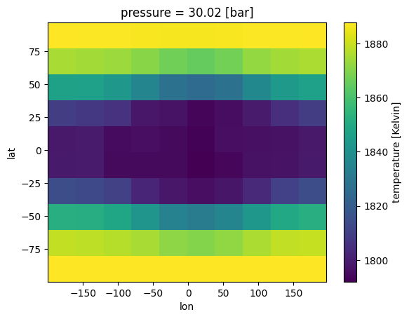
gcm_out_lores = jdi.regrid_xarray(gcm_out,num_tangle=3, latitude = np.linspace(-90, 87, 10),
                                 longitude = np.linspace(-180, 177, 10) )
gcm_out_lores['temperature'].isel(pressure=5).plot(x='lon',y='lat')
/home/nbatalh1/anaconda3/envs/pic311/lib/python3.11/site-packages/xesmf/smm.py:131: UserWarning: Input array is not C_CONTIGUOUS. Will affect performance.
  warnings.warn('Input array is not C_CONTIGUOUS. ' 'Will affect performance.')
[4]:
<matplotlib.collections.QuadMesh at 0x7f35c656ec90>
Post-process chemistry
We will use the same chemeq_3d function used previously in the 3D spectra routines
[5]:
case_3d = jdi.inputs()
case_3d.inputs['atmosphere']['profile'] = gcm_out_lores
case_3d.chemeq_3d(n_cpu=3)
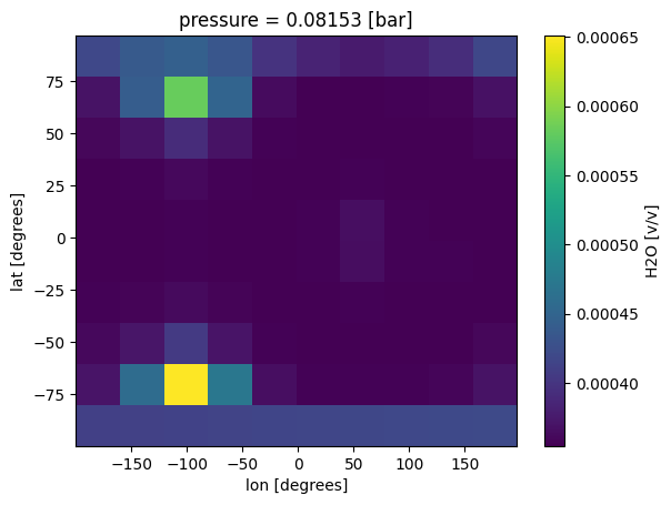
See output on generic grid you created
[6]:
case_3d.inputs['atmosphere']['profile']['H2O'].isel(pressure=30).plot(x='lon',y='lat')
[6]:
<matplotlib.collections.QuadMesh at 0x7f3800fe9090>
Add to bundle, compute phase curve
[7]:
n_phases = 4
min_phase = 0
max_phase = 2*np.pi
phase_grid = np.linspace(min_phase,max_phase,n_phases)#between 0 - 2pi
#send params to phase angle routine
case_3d.phase_angle(phase_grid=phase_grid,
num_gangle=6, num_tangle=6,calculation='thermal')
#NOTE: notice below that we are NOT submitting a dataframe , because we have already done so
#above in preparation for chemeq_3d
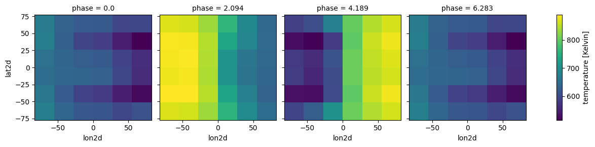
case_3d.atmosphere_4d(shift = np.zeros(n_phases),zero_point='night_transit',
plot=True,verbose=False)
/home/nbatalh1/anaconda3/envs/pic311/lib/python3.11/site-packages/xesmf/smm.py:131: UserWarning: Input array is not C_CONTIGUOUS. Will affect performance.
  warnings.warn('Input array is not C_CONTIGUOUS. ' 'Will affect performance.')

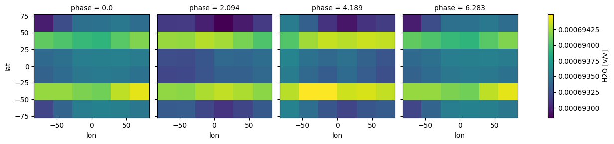
[8]:
case_3d.inputs['atmosphere']['profile']['H2O'].isel(pressure=52).plot(
                                              x='lon', y ='lat',
                                              col='phase',col_wrap=4)
[8]:
<xarray.plot.facetgrid.FacetGrid at 0x7f3800e78210>
Set gravity and stellar parameters as usual and proceed with phase curve calculation
[9]:
case_3d.gravity(radius=1,radius_unit=jdi.u.Unit('R_jup'),
                mass=1, mass_unit=jdi.u.Unit('M_jup')) #any astropy units available
case_3d.star(opacity,5000,0,4.0, radius=1, radius_unit=jdi.u.Unit('R_sun'))
allout = case_3d.phase_curve(opacity, n_cpu = 3,#jdi.cpu_count(),
                             full_output=True)
Analyze Phase Curves
Proceed with analysis as usual!
[10]:
#same old same old
wno =[];fpfs=[];legend=[]
for iphase in allout.keys():
    w,f = jdi.mean_regrid(allout[iphase]['wavenumber'],
                               allout[iphase]['fpfs_thermal'],R=100)
    wno+=[w]
    fpfs+=[f*1e6]
    legend +=[str(int(iphase*180/np.pi))]
jpi.show(jpi.spectrum(wno, fpfs, plot_width=500,legend=legend,
                     palette=jpi.pals.viridis(n_phases)))
Run Thermal Phase Curve w/ Post-Processed virga Models
Here we are putting it all together!
[11]:
#Start with you high resolution temperature, kz map
gcm_out = jdi.HJ_pt_3d(as_xarray=True,add_kz=True)
#regrid to make it more manageable, remember this is optional!
gcm_out_lores = jdi.regrid_xarray(gcm_out,num_tangle=3, latitude= np.linspace(-90, 87, 10),
longitude = np.linspace(-180, 177, 10) )
#start your picaso bundle and add your atmospheric profile
case = jdi.inputs()
#add stellar and gravity parameters
case.gravity(radius=1,radius_unit=jdi.u.Unit('R_jup'),
mass=1, mass_unit=jdi.u.Unit('M_jup')) #any astropy units available
case.star(opacity,5000,0,4.0, radius=1, radius_unit=jdi.u.Unit('R_sun'))
case.inputs['atmosphere']['profile'] = gcm_out_lores
#post-process chemistry
case.chemeq_3d(n_cpu=3)
mieff_directory = '/data/virga/'
#post-process clouds
clds = case.virga_3d(['MnS'], mieff_directory,fsed=1,kz_min=1e10,
verbose=False,full_output=True,n_cpu=1
)
#define phase angle gird
case.phase_angle(phase_grid=phase_grid,
num_gangle=6, num_tangle=6,calculation='thermal')
#create your 4th phase dimension with the shift parameter
case.atmosphere_4d(shift = np.zeros(n_phases),zero_point='night_transit',
plot=True,verbose=False)
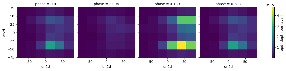
case.clouds_4d(plot=True,verbose=False)
#RUN PHASE CURVE WAHOO!!
allout = case.phase_curve(opacity, n_cpu = 3,#jdi.cpu_count(),
full_output=True)
/home/nbatalh1/anaconda3/envs/pic311/lib/python3.11/site-packages/xesmf/smm.py:131: UserWarning: Input array is not C_CONTIGUOUS. Will affect performance.
  warnings.warn('Input array is not C_CONTIGUOUS. ' 'Will affect performance.')
/home/nbatalh1/anaconda3/envs/pic311/lib/python3.11/site-packages/xesmf/smm.py:131: UserWarning: Input array is not C_CONTIGUOUS. Will affect performance.
  warnings.warn('Input array is not C_CONTIGUOUS. ' 'Will affect performance.')
Currently computing Phase (2, 4.1887902047863905)
Currently computing Phase (2, 4.1887902047863905)
Currently computing Phase (0, 0.0)
Currently computing Phase (1, 2.0943951023931953)
Currently computing Phase (1, 2.0943951023931953)
Currently computing Phase (3, 6.283185307179586)
Currently computing Phase (0, 0.0)
/home/nbatalh1/anaconda3/envs/pic311/lib/python3.11/site-packages/joblib-1.3.2-py3.11.egg/joblib/externals/loky/process_executor.py:752: UserWarning: A worker stopped while some jobs were given to the executor. This can be caused by a too short worker timeout or by a memory leak.
  warnings.warn(
[12]:
#same old same old
wno =[];fpfs=[];legend=[]
for iphase in allout.keys():
    w,f = jdi.mean_regrid(allout[iphase]['wavenumber'],
                               allout[iphase]['fpfs_thermal'],R=100)
    wno+=[w]
    fpfs+=[f*1e6]
    legend +=[str(int(iphase*180/np.pi))]
jpi.show(jpi.spectrum(wno, fpfs, plot_width=500,legend=legend,
                     palette=jpi.pals.viridis(n_phases)))