Note

Download full notebook here

Post-Process 3D Clouds Input

There are many cases were you may want to post-process components from a 3D GCM output. Post-processing is used to compensate for simplicities, or assumptions within a GCM. For example, you may want to post-process clouds on your output spectra, even if your initial GCM run did not include the effects of clouds.

In this notebook you will learn: 1. How to post- process clouds using simple box model 2. How to post- process clouds using virga

You should already know: 1. How to format and regrid an xarray dataset

Next notebook you will learn: 1. How to create spectra and phase curves from 3D input

import pandas as pd
import numpy as np
import xarray as xr

from picaso import justdoit as jdi
from picaso import justplotit as jpi

gcm_out =  jdi.HJ_pt_3d(as_xarray=True)

Post-Process Clouds: User Options

1. User-defined input: this would only be used to explore simplistic cases (e.g. 100% H2O, or 50/50 H2/H2O). It also might be the case that you have abundance models from elsewhere (e.g. 3D model or GCM) and want to add it to your pressure/temperature xarray

2. Computationally intensive route: Usually GCM output is at a very high spatial resolution – higher than what is needed to post-process spectra. If you want, you can grab chemistry for every single lat x lon point in your grid first. Then, regrid after.

   • Pro: you would only have to run it once, then you could regrid to different spatial resolutions later.

   • Con: computationally expensive (e.g. 128 x 64 pts x ~1 second = 2 hours per model .. though the exact time depends on how many altitude points you have)

3. Computationally efficient route: Regrid first, then compute chemistry.

   • Pro: would save potentially hundreds of chemistry computations

   • Con: if you aren’t happy with your initial binning choice, you may have to repeat the calculation a few times to get it right

In this demo, we will do option #1 and #3 so that it can be self-contained and computationally fast, but you should explore what works best for your problem.

Post-Process Clouds: User Defined Input

Very similar to chemistry process, we can create an xarray that has our cloud output. Note that for clouds there is a fourth dimension (wavelength)

# create coords
lon = gcm_out.coords.get('lon').values
lat = gcm_out.coords.get('lat').values
pres = gcm_out.coords.get('pressure').values
wno_grid = np.linspace(1e4/2,1e4/1,10)#cloud properties are defined on a wavenumber grid

#create box-band cloud model
fake_opd = np.zeros((len(lon), len(lat),len(pres), len(wno_grid))) # create fake data
where_lat = np.where(((lat>-50) & (lat<50)))#creating a grey cloud band
where_pres = np.where(((pres<0.01) & (pres>.001)))#creating a grey cloud band
for il in where_lat[0]:
    for ip in where_pres[0]:
        fake_opd[:,il,ip,:]=10 #optical depth of 10 (>>1)

#make up asymmetry and single scattering properties
fake_asymmetry_g0 = 0.8+ np.zeros((len(lon), len(lat),len(pres), len(wno_grid)))
fake_ssa_w0 = 0.9+ np.zeros((len(lon), len(lat),len(pres), len(wno_grid)))

# put data into a dataset
ds_cld= xr.Dataset(
    data_vars=dict(
        opd=(["lon", "lat","pressure","wno"], fake_opd,{'units': 'depth per layer'}),
        g0=(["lon", "lat","pressure","wno"], fake_asymmetry_g0,{'units': 'none'}),
        w0=(["lon", "lat","pressure","wno"], fake_ssa_w0,{'units': 'none'}),
    ),
    coords=dict(
        lon=(["lon"], lon,{'units': 'degrees'}),#required
        lat=(["lat"], lat,{'units': 'degrees'}),#required
        pressure=(["pressure"], pres,{'units': 'bar'}),#required
        wno=(["wno"], wno_grid,{'units': 'cm^(-1)'})#required for clouds
    ),
    attrs=dict(description="coords with vectors"),
)

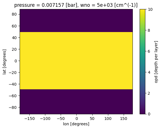
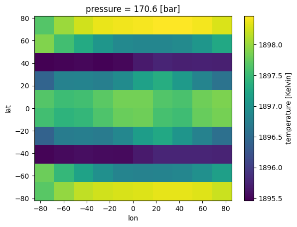
Visualize Cloud Input

ds_cld['opd'].isel(pressure=where_pres[0][0],wno=0).plot(x='lon',y='lat')

<matplotlib.collections.QuadMesh at 0x7f284b723410>

Add clouds to picaso bundle

As a recap, in the steps below we: 1. Initiate a new run (jdi.inputs) 2. Define the geometry of the run (phase_angle) 3. Set the pressure-temperature-lat-lon profile (atmosphere_3d)

Note here we are not worrying about chemical abundances (see post process chem tutorial). We will combine both clouds and chemistry steps in the next tutorial on 3D Spectra.

#first step is identical to what's been done in the past
case_3d = jdi.inputs()
case_3d.phase_angle(0, num_tangle=4, num_gangle=4)
#turning off alerts since we already went through this
case_3d.atmosphere_3d(gcm_out, regrid=True, plot=False,verbose=False)

/home/nbatalh1/anaconda3/envs/pic311/lib/python3.11/site-packages/xesmf/smm.py:131: UserWarning: Input array is not C_CONTIGUOUS. Will affect performance.
  warnings.warn('Input array is not C_CONTIGUOUS. ' 'Will affect performance.')

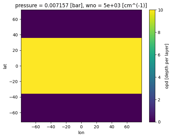
Now we can add cloud box model, which will be automatically regridded to the inputs based on the phase_angle function ran above

case_3d.clouds_3d(ds_cld,iz_plot=where_pres[0][0])

verbose=True;regrid=True; Regridding 3D output to ngangle=4, ntangle=4, with phase=0.

/home/nbatalh1/anaconda3/envs/pic311/lib/python3.11/site-packages/xesmf/smm.py:131: UserWarning: Input array is not C_CONTIGUOUS. Will affect performance.
  warnings.warn('Input array is not C_CONTIGUOUS. ' 'Will affect performance.')

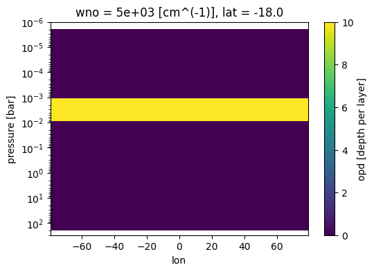
Stylize plots to see reversed pressure axis in log

fig, ax = jpi.plt.subplots(figsize=(6, 4))
case_3d.inputs['clouds']['profile']['opd'].isel(
    lat=2,wno=0).plot(
    x='lon',y='pressure',ax=ax)
ax.set_ylim([3e2,1e-6])
ax.set_yscale('log')

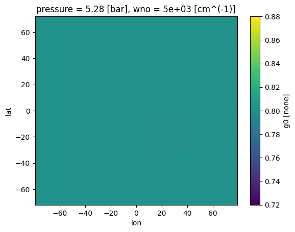
See other regridded variables

All the elements of your data bundle have been regridded! Though for now this is not too interesting since we have set the asymmetry to a constant value of 0.8

case_3d.inputs['clouds']['profile']['g0'].isel(pressure=10,wno=0).plot(
    x='lon',y='lat')

<matplotlib.collections.QuadMesh at 0x7f283de17bd0>

Post-Process Clouds: virga cloud model

We will run this example on a very coarse (5x5) grid to make it faster. Note that similar to the chemeq_3d routine, running virga_3d will just run nganglexntangle 1d models. There is no transport of particles in the vertical/horizontal direction.

NOTE!! If you are not familiar with virga models it is highly recommended that you start in one-dimension first. You can review the tutorials here. This tutorial will not explain the required virga inputs.

opacity = jdi.opannection(wave_range=[1,2])
gcm_out =  jdi.HJ_pt_3d(as_xarray=True,add_kz=True)
case_3d = jdi.inputs()
case_3d.phase_angle(0, num_tangle=10, num_gangle=10)
case_3d.atmosphere_3d(gcm_out, regrid=True)
case_3d.gravity(radius=1,radius_unit=jdi.u.Unit('R_jup'),
                mass=1, mass_unit=jdi.u.Unit('M_jup')) #any astropy units available
case_3d.star(opacity,5000,0,4.0, radius=1, radius_unit=jdi.u.Unit('R_sun'))

verbose=True;regrid=True; Regridding 3D output to ngangle=10, ntangle=10, with phase=0.

/home/nbatalh1/anaconda3/envs/pic311/lib/python3.11/site-packages/xesmf/smm.py:131: UserWarning: Input array is not C_CONTIGUOUS. Will affect performance.
  warnings.warn('Input array is not C_CONTIGUOUS. ' 'Will affect performance.')

Run Virga!

mieff_directory = '/data/virga/'
clds = case_3d.virga_3d(['MnS'], mieff_directory,fsed=1,kz_min=1e10,
                        verbose=False,n_cpu=3, full_output=True
                       )

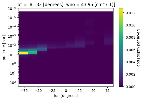
Plot optical depth as a function of longitude

fig, ax = jpi.plt.subplots(figsize=(6, 4))
case_3d.inputs['clouds']['profile']['opd'].isel(lat=5,wno=0).plot(
    x='lon',y='pressure',ax=ax)
ax.set_ylim([3e2,1e-6])
ax.set_yscale('log')

Trouble Shooting Negative Kz Values (smooth_kz)

GCM runs produce both positive and negative K_z values. A negative K_z represents downdrafts, which cannot be accounted for in virga. In fact, virga has a default minimum value of 1e5 cm\(^2\)/s. For the above run, note I used a very large kz_min value of 1e10cm\(^2\)/s. The smaller the k_z value, the values create small particles. Let’s take at some of the difficulty with smoothing over K_z profiles:

gcm_out =  jdi.HJ_pt_3d(as_xarray=True,add_kz=True)
test = jdi.inputs()
test.phase_angle(0, num_tangle=10, num_gangle=10)
test.atmosphere_3d(gcm_out, regrid=True, verbose=False, plot=False)

/home/nbatalh1/anaconda3/envs/pic311/lib/python3.11/site-packages/xesmf/smm.py:131: UserWarning: Input array is not C_CONTIGUOUS. Will affect performance.
  warnings.warn('Input array is not C_CONTIGUOUS. ' 'Will affect performance.')

Explore some profiles in our 3d Kz grid

jpi.output_notebook()
df = test.inputs['atmosphere']['profile'].isel(lon=0, lat=0
                            ).to_pandas(
                            ).reset_index(
                            ).drop(
                            ['lat','lon'],axis=1
                            ).sort_values('pressure')

fig = jpi.figure(y_axis_type='log',y_range=[1e2,1e-6],x_axis_label='Kz (cm2/s)',
                 y_axis_label='pressure (bars)',
                 width=300, height=300, x_range=[-1e11, 1e11])
fig.line(df['kz']*1e4,df['pressure'])
jpi.show(fig)

Loading BokehJS ...

Experiment with splines

x=np.log10(df['pressure'].values)
df['logp']=x
y = np.log10(df['kz'].values)
x=x[y>0]
y = y[y>0]
spl = jdi.UnivariateSpline(x, y,ext=3)
df['splKz'] = spl(np.log10(df['pressure'].values))

/tmp/ipykernel_110649/2109147401.py:3: RuntimeWarning: invalid value encountered in log10
  y = np.log10(df['kz'].values)

fig = jpi.figure(y_axis_type='log',y_range=[1e2,1e-6], x_axis_type='log',
                 x_axis_label='Kz (cm2/s)',
                 y_axis_label='pressure (bars)',
                 width=300, height=300, x_range=[1e5, 1e11])
fig.line(df['kz']*1e4,df['pressure'])
fig.line(10**df['splKz']*1e4, df['pressure'],color='red')
fig.circle(10**y*1e4, 10**x,color='red',size=7)
jpi.show(fig)