Spherical Integration in PICASO
In this tutorial you will learn the different integration schemes that exist within PICASO.
[1]:
import warnings
warnings.filterwarnings('ignore')
import numpy as np
import pandas as pd
import astropy.units as u

#picaso
import picaso.opacity_factory as opa_fa
from picaso import justdoit as jdi
from picaso import justplotit as jpi
#plotting
from bokeh.io import output_notebook

output_notebook()
from bokeh.plotting import show,figure
Test Geometry with Brown Dwarf Sonora Example
Let’s try three different cases
[2]:
wave_range = [3,5]

opa = jdi.opannection(wave_range=wave_range)

case1 = jdi.inputs(calculation='browndwarf')

case2 = jdi.inputs(calculation='browndwarf')

case3 = jdi.inputs(calculation='browndwarf')
First case will be a full 10x10 grid, second will be the same 10x10 grid but leveraging symmetry, last will be a 1x10 grid. A 1x10 grid automaticlly leverages symmetry as we will see in the disco plots below.
[3]:
names = ['10x10', '10x10sym', '1x10']
cases = [ case1, case2, case3]#, case5]

case1.phase_angle(num_tangle=10, num_gangle=10)
case2.phase_angle(num_tangle=10, num_gangle=10, symmetry=True)
case3.phase_angle(num_tangle=1, num_gangle=10) #remember num_tangle=1 automatically insinuates symmetry
Query from Sonora Profile Grid
(Same as before) Download the profile files that are located in the profile.tar file
Once you untar the file you can set the file path below. You do not need to unzip each profile. picaso will do that upon read in. picaso will find the nearest neighbor and attach it to your class.
[4]:
# Note here that we do not need to provide case.star, since there is none!
for i in cases:i.gravity(gravity=100 , gravity_unit=u.Unit('m/s**2'))

#grab sonora profile
sonora_profile_db = '/data/sonora_profile/'
Teff = 900
#this function will grab the gravity you have input above and find the nearest neighbor with the
#note sonora chemistry grid is on the same opacity grid as our opacities (1060).
for i in cases:i.sonora(sonora_profile_db, Teff)
Run Spectrum
[5]:
df = {}
for i,ikey in zip(cases, names):
    print(ikey)
    df[ikey] = i.spectrum(opa, full_output=True)
10x10
10x10sym
1x10
Convert Units and Regrid
[6]:
for i,ikey in zip(cases, names):
    print(ikey)
    x,y = df[ikey]['wavenumber'], df[ikey]['thermal'] #units of erg/cm2/s/cm
    xmicron = 1e4/x

    flamy = y*1e-8 #per anstrom instead of per cm
    sp = jdi.psyn.ArraySpectrum(xmicron, flamy,
                                waveunits='um',
                                fluxunits='FLAM')
    sp.convert("um")
    sp.convert('Fnu') #erg/cm2/s/Hz

    x = sp.wave #micron
    y= sp.flux #erg/cm2/s/Hz
    df[ikey]['fluxnu'] = y
    x,y = jdi.mean_regrid(1e4/x, y, R=300) #wavenumber, erg/cm2/s/Hz
    df[ikey]['regridy'] =  y
    df[ikey]['regridx'] = x
10x10
10x10sym
1x10
Compare Different Integration Schemes with Sonora Grid
[7]:
son = pd.read_csv('sp_t900g100nc_m0.0',delim_whitespace=True,
                 skiprows=3,header=None,names=['w','f'])
sonx, sony =  jdi.mean_regrid(1e4/son['w'], son['f'], newx=x)
[8]:
to_compare = []
fraction_compare = []
for ikey in names:
    to_compare += [df[ikey]['regridy']]
    fraction_compare += [df[ikey]['regridy']/sony]
[9]:
to_compare += [sony]
legend_label = names + ['sonora']
Compare Accuracy of Different Number of Integration Points
[10]:
show(jpi.spectrum([x]*len(to_compare),to_compare, legend=legend_label
                  ,plot_width=800,x_range=wave_range,y_axis_type='log'))
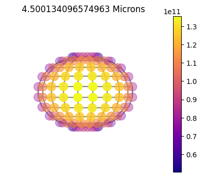
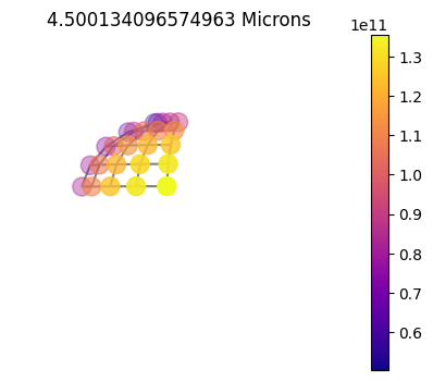
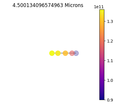
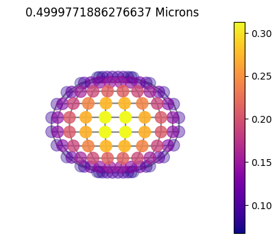
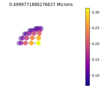
Visualize Integration Schemes
[11]:
for ikey in names:
    asdict = df[ikey]['full_output']
    print(ikey)
    jpi.disco(asdict, calculation='thermal', wavelength=[4.5])
10x10
10x10sym
1x10
Plot Gauss Weights
Plotting out the gauss weights you can see the difference between the purely 1D (without using chebyshev weights), 2D full grid and 2D symmetric.
[12]:
fig = figure(height=300, x_axis_label='gangle',y_axis_label='gweight')
for i in [fig.line, fig.circle]: i(cases[0].inputs['disco']['gangle'],
         cases[0].inputs['disco']['gweight'],color='red',
                                  legend_label=names[0]  )

for i in [fig.line, fig.circle]: i(cases[1].inputs['disco']['gangle'],
         cases[1].inputs['disco']['gweight'],color='blue',
                                 legend_label=names[1] )

for i in [fig.line, fig.circle]: i(cases[2].inputs['disco']['gangle'],
         cases[2].inputs['disco']['gweight']
                                   ,color='green',legend_label=names[2])


show(fig)
Geometry with Reflectivity and Non-Zero Phase
In this example, let’s look at four difference cases.
1x10 symmetric grid with zero phase (inherently symmetric)
10x10 grid with zero phase but let’s run without symmetry utilization
same as 2 but flipping on symmetry
Non-zero phase, full grid
[13]:
wave_range = [0.3,1]

opa = jdi.opannection(wave_range=wave_range)

case1 = jdi.inputs()
case2 = jdi.inputs()
case3 = jdi.inputs()
case4 = jdi.inputs()
[14]:
names = ['1x10','10x10', '10x10sym',  '10x10_60']

case1.phase_angle(phase=0, num_tangle=1, num_gangle=10) #remember num_tangle=1 automatically insinuates symmetry
case2.phase_angle(phase=0, num_tangle=10, num_gangle=10)
case3.phase_angle(phase=0, num_tangle=10, num_gangle=10, symmetry=True)
case4.phase_angle(phase=60*np.pi/180, num_tangle=10, num_gangle=10)

cases = [ case1, case2, case3, case4]
[15]:
for i in cases:i.gravity(gravity=20 , gravity_unit=u.Unit('m/s**2'))
for i in cases:i.atmosphere(filename = jdi.jupiter_pt(), delim_whitespace=True)
for i in cases:i.approx(raman='pollack')
for i in cases:i.star(opa, 5000,0,4.0)
[16]:
df = {}
for i,ikey in zip(cases, names):
    print(ikey)
    df[ikey] = i.spectrum(opa,calculation='reflected' ,full_output=True)
1x10
10x10
10x10sym
10x10_60
[17]:
to_compare = []
fraction_compare = []
for ikey in names:
    x,y = df[ikey]['wavenumber'], df[ikey]['albedo']
    x,y = jdi.mean_regrid(x, y, R=100) #wavenumber, erg/cm2/s/Hz
    df[ikey]['regridy'] =  y
    df[ikey]['regridx'] = x
    to_compare += [df[ikey]['regridy']]
[18]:
show(jpi.spectrum([x]*len(to_compare),to_compare, legend=names
                  ,plot_width=800))
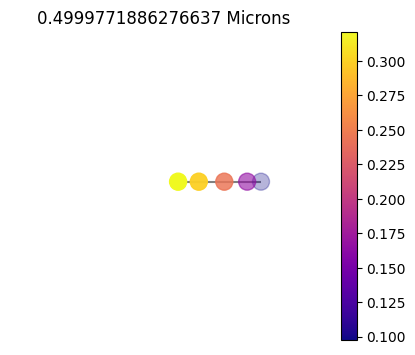
If you zoom in, you will notice that the 1x10 is just slightly off the full 10x10 grid. This is certainly not enough to warrant doing a full 10x10=100 calculations opposed to the 10/2x1=5 calculations it too to run the 1x10 grid (you can see what RT points were ran below).
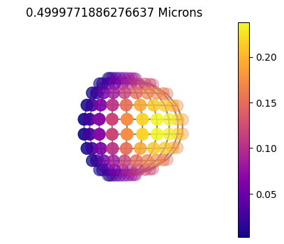
[19]:
for ikey in names:
    asdict = df[ikey]['full_output']
    print(ikey)
    jpi.disco(asdict, calculation='reflected', wavelength=[0.5])
1x10
10x10
10x10sym
10x10_60
[ ]: