Table of Contents
1 Handling 3D Inputs with PICASO
1.1 xarray tutorial: Convert numpy arrays to xarray DataSet
1.2 xarray tutorial: Easy plotting
1.3 xesfm tutorial: Step-by-step regrid 3D GCM
1.4 Regrid 3D GCM with PICASO
Handling 3D Inputs with PICASO
Many GCM groups have their files stored as netCDF files. Therefore, you may already be used to xarray format. If that is the case you will be able to directly input your xarray formatted data to PICASO to get out post-processed spectra. If not though, this tutorial will walk you through how to structure your data in xarray format.
What you will learn:
How to convert traditional numpy arrays to
xarrayformatted data, which is common for 3D GCM outputHow to regrid using
xarrayandxesmf’sregridderHow to use
PICASObuilt in function (which use #2)
[1]:
import pandas as pd
import numpy as np

from picaso import justdoit as jdi
Two new packages you will need, that are not required components of other models: xesmf and xarray. You can read more about the installing these packages here:
Install XESMF - will only be needed if you want to use their really handy regridding tools
Install xarray - needed for all PICASO 3d operations
[2]:
import xesmf as xe
import xarray as xr
We will begin with an example file from the MIT GCM group (courtesy of Tiffany Kataria).
[3]:
gcm_out = jdi.HJ_pt_3d()
We are going to go through the motions of converting basic numpy arrays to xarray format. If you already understand xarrays you may skip to the `picaso section <#regrid-3d-gcm-with-picaso>`__
[4]:
gcm_out.keys()
[4]:
dict_keys(['pressure', 'temperature', 'kzz', 'latitude', 'longitude'])
In this example, pressure, temperature, and kzz are all on a coordinate system that is :
n_longitude (128) x n_latitude (64) x n_pressure (53)
[5]:
gcm_out['temperature'].shape, len(gcm_out['longitude']), len(gcm_out['latitude'])
[5]:
((128, 64, 53), 128, 64)
xarray tutorial: Convert numpy arrays to xarray DataSet
The comments with required next to them indicate that they are required for picaso to create a spectrum
[6]:
# create data
data = gcm_out['temperature']

# create coords
lon = gcm_out['longitude']
lat = gcm_out['latitude']
pres = gcm_out['pressure'][0,0,:]

# put data into a dataset
ds = xr.Dataset(
    data_vars=dict(
        temperature=(["lon", "lat","pressure"], data,{'units': 'Kelvin'})#, required
        #kzz = (["x", "y","z"], gcm_out['kzz'])#could add other data components if wanted
    ),
    coords=dict(
        lon=(["lon"], lon,{'units': 'degrees'}),#required
        lat=(["lat"], lat,{'units': 'degrees'}),#required
        pressure=(["pressure"], pres,{'units': 'bar'})#required*
    ),
    attrs=dict(description="coords with vectors"),
)
[7]:
ds
[7]:
<xarray.Dataset> Size: 3MB
Dimensions:      (lon: 128, lat: 64, pressure: 53)
Coordinates:
  * lon          (lon) float64 1kB -180.0 -177.2 -174.4 ... 171.6 174.4 177.2
  * lat          (lat) float64 512B -90.0 -87.19 -84.38 ... 81.56 84.38 87.19
  * pressure     (pressure) float64 424B 170.6 120.5 ... 3.42e-06 2.416e-06
Data variables:
    temperature  (lon, lat, pressure) float64 3MB 1.896e+03 1.809e+03 ... 750.7
Attributes:
description: coords with vectorsxarray tutorial: Easy plotting
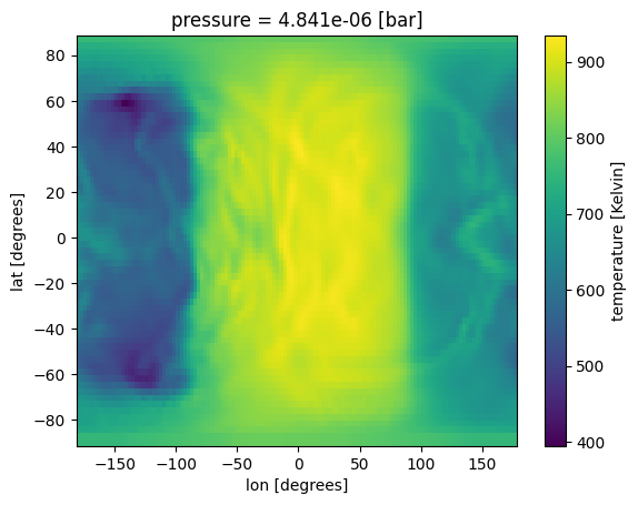
[8]:
ds['temperature'].isel(pressure=50).plot(x='lon',y='lat')
[8]:
<matplotlib.collections.QuadMesh at 0x7fe688d22b10>
xesmf tutorial: Step-by-step regrid 3D GCM
The biggest complication with moving to 3D is making sure that the latitude/longitude grids of some users GCM and picaso line up properly. picaso computes a flux integration on specific gauss and tchebychev angles. Meaning, your GCM input will need to be regridded to fit our angles. Luckily, as you will see below, it is very easy to do this!
First, we will show you how this is done using xesmf, then we will introduce the PICASO function that leverages these same techniques.
Step 1) Get latitude/longitude grid used by picaso
Gauss angles are essentially equivalent to lonGitudes
Tchebychev angles are essentially equivalent to laTitudes.
[9]:
n_gauss_angles =10
n_chebychev_angles=10

gangle, gweight, tangle, tweight = jdi.get_angles_3d(n_gauss_angles, n_chebychev_angles)
ubar0, ubar1, cos_theta, latitude, longitude = jdi.compute_disco(n_gauss_angles, n_chebychev_angles, gangle, tangle, phase_angle=0)
Step 2) Create the xesmf regridder
[10]:
ds_out = xr.Dataset({'lon': (['lon'], longitude*180/np.pi),
                     'lat': (['lat'], latitude*180/np.pi),
                    }
                   )

regridder = xe.Regridder(ds, ds_out, 'bilinear')
ds_out = regridder(ds,keep_attrs=True)
/home/nbatalh1/anaconda3/envs/pic311/lib/python3.11/site-packages/xesmf/smm.py:131: UserWarning: Input array is not C_CONTIGUOUS. Will affect performance.
  warnings.warn('Input array is not C_CONTIGUOUS. ' 'Will affect performance.')
All done!
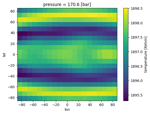
[11]:
ds_out['temperature'].isel(pressure=10).plot(x='lon', y ='lat')
[11]:
<matplotlib.collections.QuadMesh at 0x7fe67ab0d810>
Regrid 3D GCM with PICASO
The above code is all the PICASO built in function does – in addition to completing some checks to make sure that your model run is on the same grid as what you are wanting PICASO run.
[12]:
ds = jdi.HJ_pt_3d(as_xarray=True)
DIY Option 1
For completeness, first here is the function picaso uses internally. You might use this if you want to manipulate results before supplying picaso with your final input.
[13]:
#regrid yourself
out_ds = jdi.regrid_xarray(ds, num_gangle=20,
                               num_tangle=20, phase_angle=0)
#then supply to picaso
case_3d = jdi.inputs()
case_3d.phase_angle(0, num_gangle=20, num_tangle=20)

#here, regrid is false because you have already done it yourself
case_3d.atmosphere_3d(out_ds,regrid=False,plot=True,verbose=True)
/home/nbatalh1/anaconda3/envs/pic311/lib/python3.11/site-packages/xesmf/smm.py:131: UserWarning: Input array is not C_CONTIGUOUS. Will affect performance.
  warnings.warn('Input array is not C_CONTIGUOUS. ' 'Will affect performance.')
verbose=True;Only one data variable included. Make sure to add in chemical abundances before trying to run spectra.

Easiest Option 2
Use the regular PICASO workflow to regrid your 3d input
[14]:
case_3d = jdi.inputs()
case_3d.phase_angle(0, num_gangle=20, num_tangle=20)
#regrid is True as you will do it within the function
case_3d.atmosphere_3d(ds,regrid=True,plot=True,verbose=True)
verbose=True;regrid=True; Regridding 3D output to ngangle=20, ntangle=20, with phase=0.
verbose=True;Only one data variable included. Make sure to add in chemical abundances before trying to run spectra.
We have solved regridding our temperature-pressure profile. However, PICASO has notified us of another step we must take before running a spectrum: verbose=True;Only one data variable included. Make sure to add in chemical abundances before trying to run spectra.
In the next notebook you will see how to add chemistry and/or clouds to your 3D input.