One-Dimensional Climate Models: The Basics of Planets
In this tutorial you will learn the very basics of running 1D climate runs. For a more in depth look at the climate code check out Mukherjee et al. 2022 (note this should also be cited if using this code/tutorial).
What you should already be familiar with:
What you will need to download to use this tutorial:
Download 196 Correlated-K Tables from Roxana Lupu to be used by the climate code for opacity (if you completed the brown dwarf tutorial you should already have this)
Note: the two files above are dependent on metallicity and C/O.
[1]:
import warnings
warnings.filterwarnings('ignore')
import picaso.justdoit as jdi
import picaso.justplotit as jpi
import astropy.units as u
import numpy as np
import matplotlib.pyplot as plt
%matplotlib inline
[2]:
#1 ck tables from roxana
mh = '+100'#'+1.0' #log metallicity, 10xSolar
CtoO = '100'#'1.0' # CtoO ratio, Solar C/O
ck_db = f'/data/kcoeff_2020_v3/sonora_2020_feh{mh}_co_{CtoO}.data.196'
[3]:
# Notice The keyword ck is set to True because you want to use the correlated-k opacities for your calculation
# and not the line by line opacities
opacity_ck = jdi.opannection(ck_db=ck_db) # grab your opacities
Starting up the Run
You will notice that starting a run is nearly identical as running a spectrum and brown dwarf climate model. However, how we will add climate=True to our inputs flag. We will also specify planet in this case, which will turn on the irradiation the object is receiving.
New Parameter (was also used in the Brown Dwarf tutorial): Effective Temperature. This excerpt from Modeling Exoplanetary Atmospheres (Fortney et al) provides a thorough description and more reading, if you are interested.
If the effective temperature, \(T_{eff}\), is defined as the temperature of a blackbody of the same radius that would emit the equivalent flux as the real planet, \(T_{eff}\) and \(T_{eq}\) can be simply related. This relation requires the inclusion of a third temperature, \(T_{int}\), the intrinsic effective temperature, that describes the flux from the planet’s interior. These temperatures are related by:
\(T_{eff}^4 = T_{int}^4 + T_{eq}^4\)
We then recover our limiting cases: if a planet is self-luminous (like a young giant planet) and far from its parent star, \(T_{eff} \approx T_{int}\); for most rocky planets, or any planets under extreme stellar irradiation, \(T_{eff} \approx T_{eq}\).
[4]:
cl_run = jdi.inputs(calculation="planet", climate = True) # start a calculation

#note you need to put the climate keyword to be True in order to do so
# now you need to add these parameters to your calculation


tint= 200 # Intrinsic Temperature of your Planet in K
grav = 4.5 # Gravity of your Planet in m/s/s

cl_run.gravity(gravity=grav, gravity_unit=u.Unit('m/(s**2)')) # input gravity
cl_run.effective_temp(tint) # input effective temperature
Let’s now input the host-star properties
[5]:
T_star =5326.6 # K, star effective temperature
logg =4.38933 #logg , cgs
metal =-0.03 # metallicity of star
r_star = 0.932 # solar radius
semi_major = 0.0486 # star planet distance, AU

cl_run.star(opacity_ck, temp =T_star,metal =metal, logg =logg, radius = r_star,
            radius_unit=u.R_sun,semi_major= semi_major , semi_major_unit = u.AU)#opacity db, pysynphot database, temp, metallicity, logg
Initial T(P) Guess
Every calculation requires an initial guess of the pressure temperature profile. The code will iterate from there to find the correct solution. A few tips:
We recommend using typically 51-91 atmospheric pressure levels. Too many pressure layers increases the computational time required for convergence. Too little layers makes the atmospheric grid too coarse for an accurate calculation.
Start with a guess that is close to your expected solution. One easy way to get fairly close is by using the Guillot et al 2010 temperature-pressure profile approximation
[6]:
nlevel = 91 # number of plane-parallel levels in your code

#Lets set the max and min at 1e-4 bars and 500 bars
Teq=1000 # planet equilibrium temperature
pt = cl_run.guillot_pt(Teq, nlevel=nlevel, T_int = tint, p_bottom=2, p_top=-6)
temp_guess = pt['temperature'].values
pressure = pt['pressure'].values
Initial Convective Zone Guess
You also need to have a crude guess of the convective zone of your atmosphere. Generally the deeper atmosphere is always convective. Again a good guess is always the published SONORA grid of models for this. But lets assume that the bottom 7 levels of the atmosphere is convective.
New Parameters:
nofczns: Number of convective zones. Though the code has functionality to solve for more than one. In this basic tutorial, let’s stick to 1 for now.rfacv: (See Mukherjee et al Eqn. 20r_st) https://arxiv.org/pdf/2208.07836.pdf
Non-zero values of rst (aka “rfacv” legacy terminology) is only relevant when the external irradiation on the atmosphere is non-zero. In the scenario when a user is computing a planet-wide average T(P) profile, the stellar irradiation is contributing to 50% (one hemisphere) of the planet and as a result rst = 0.5. If instead the goal is to compute a night-side average atmospheric state, rst is set to be 0. On the other extreme, to compute the day-side atmospheric state of a tidally locked planet rst should be set at 1.
[7]:
nofczns = 1 # number of convective zones initially. Let's not play with this for now.

nstr_upper = 85 # top most level of guessed convective zone
nstr_deep = nlevel -2 # this is always the case. Dont change this
nstr = np.array([0,nstr_upper,nstr_deep,0,0,0]) # initial guess of convective zones

# Here are some other parameters needed for the code.
rfacv = 0.5 #we are focused on a brown dwarf so let's keep this as is
Now we would use the inputs_climate function to input everything together to our cl_run we started.
[8]:
cl_run.inputs_climate(temp_guess= temp_guess, pressure= pressure,
                      nstr = nstr, nofczns = nofczns , rfacv = rfacv)
Run the Climate Code
The actual climate code can be run with the cl_run.run command. The save_all_profiles is set to True to save the T(P) profile at all steps. The code will now iterate from your guess to reach the correct atmospheric solution for your brown dwarf of interest.
[9]:
out = cl_run.climate(opacity_ck, save_all_profiles=True,with_spec=True)
Iteration number  0 , min , max temp  858.7819362235995 2288.0492302028547 , flux balance  -31.73873302691932
Iteration number  1 , min , max temp  833.7793860808221 2745.5897658916588 , flux balance  17.402430972236605
Iteration number  2 , min , max temp  832.5640577698005 2632.5257722176316 , flux balance  0.2574682862204917
Iteration number  3 , min , max temp  832.5555399341288 2620.6543717701484 , flux balance  0.001234890146788473
Iteration number  4 , min , max temp  832.5554966773734 2620.5050759851515 , flux balance  5.739158464062829e-06
In t_start: Converged Solution in iterations  4
Big iteration is  832.5554966773734 0
Iteration number  0 , min , max temp  831.329994689357 2715.035437848504 , flux balance  -2.0023093581666105
Iteration number  1 , min , max temp  830.1622647543361 2785.2102375881227 , flux balance  0.11641005895196467
Iteration number  2 , min , max temp  830.1537154588228 2782.176490117008 , flux balance  0.0006508259035178412
In t_start: Converged Solution in iterations  2
Big iteration is  830.1537154588228 1
Iteration number  0 , min , max temp  829.9124059744206 2878.966719467169 , flux balance  0.007788429690421891
Iteration number  1 , min , max temp  829.9111443845821 2873.72098389157 , flux balance  5.221970120168576e-05
In t_start: Converged Solution in iterations  1
Big iteration is  829.9111443845821 2
Iteration number  0 , min , max temp  829.9441619449865 2929.9708193294446 , flux balance  0.0003277030604651063
Iteration number  1 , min , max temp  829.9443121662235 2928.2636306613163 , flux balance  2.8731787238920628e-06
In t_start: Converged Solution in iterations  1
Profile converged before itmx
Iteration number  0 , min , max temp  830.0677996537182 2960.4877282606344 , flux balance  0.00020125877998476374
Iteration number  1 , min , max temp  830.0684316983014 2959.9665748368416 , flux balance  9.939270944240924e-07
In t_start: Converged Solution in iterations  1
Big iteration is  830.0684316983014 0
Iteration number  0 , min , max temp  830.1717739082255 2978.180705100826 , flux balance  7.152985882966919e-05
Iteration number  1 , min , max temp  830.172289967385 2978.029321258105 , flux balance  3.381990803379245e-07
In t_start: Converged Solution in iterations  1
Profile converged before itmx
Move up two levels
Iteration number  0 , min , max temp  830.2411418494598 2787.3393255901165 , flux balance  1.4256936451967332e-05
In t_start: Converged Solution in iterations  0
Big iteration is  830.2411418494598 0
Iteration number  0 , min , max temp  830.2860537194981 2787.3404905593757 , flux balance  1.5055435081772502e-06
In t_start: Converged Solution in iterations  0
Profile converged before itmx
final [ 0 83 89  0  0  0]
Iteration number  0 , min , max temp  830.314429144484 2787.341323191593 , flux balance  -1.451567740374381e-06
In t_start: Converged Solution in iterations  0
Big iteration is  830.314429144484 0
Iteration number  0 , min , max temp  830.3325623924928 2787.3416081653627 , flux balance  -1.734531951216731e-06
In t_start: Converged Solution in iterations  0
Profile converged before itmx
YAY ! ENDING WITH CONVERGENCE
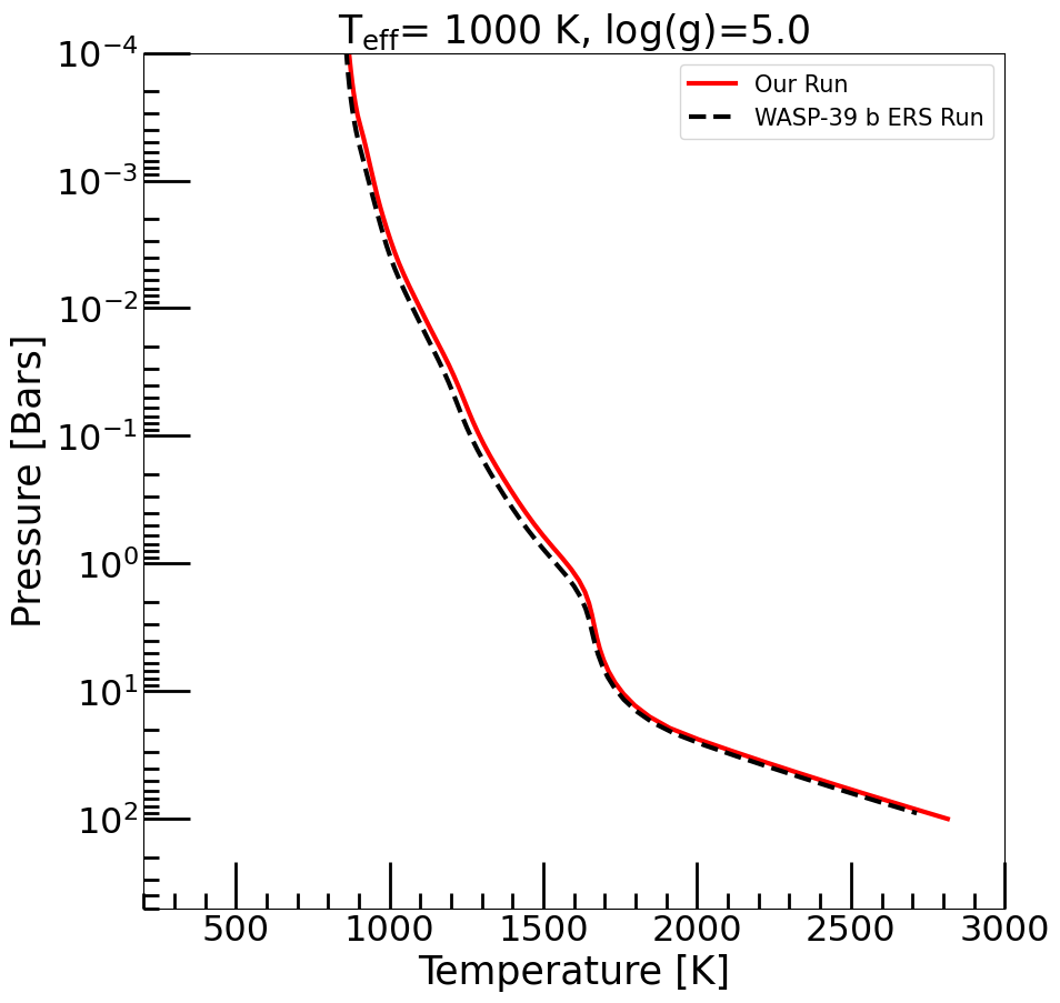
[10]:
base_case = jdi.pd.read_csv(jdi.HJ_pt(), delim_whitespace=True)

plt.figure(figsize=(10,10))
plt.ylabel("Pressure [Bars]", fontsize=25)
plt.xlabel('Temperature [K]', fontsize=25)
plt.ylim(500,1e-4)
plt.xlim(200,3000)

plt.semilogy(out['temperature'],out['pressure'],color="r",linewidth=3,label="Our Run")

plt.semilogy(base_case['temperature'],base_case['pressure'],color="k",linestyle="--",linewidth=3,label="WASP-39 b ERS Run")


plt.minorticks_on()
plt.tick_params(axis='both',which='major',length =30, width=2,direction='in',labelsize=23)
plt.tick_params(axis='both',which='minor',length =10, width=2,direction='in',labelsize=23)

plt.legend(fontsize=15)

plt.title(r"T$_{\rm eff}$= 1000 K, log(g)=5.0",fontsize=25)
[10]:
Text(0.5, 1.0, 'T$_{\\rm eff}$= 1000 K, log(g)=5.0')
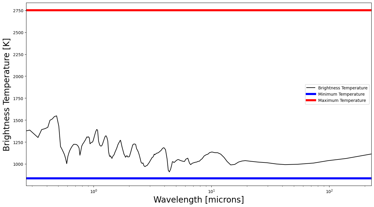
Brightness Temperature
Checking the brightness temperature serves many useful purposes:
Intuition building. Allows you to see what corresponding temperature are you sensitive to at each wavelength
Note that this temperature doesn’t need to be the physical temperature of your atmosphere but if you can find the physical converged atmospheric temperature closest to this brightness temperature you can also get an idea of the atmospheric pressure from where the flux you are seeing is originating from.
Determining if your choice in bottom boundary pressure grid was correct.
If your brightness temperature is such that you bottom out at the temperature corresponding to the highest pressure, you have not extended your grid to high enough pressures.
Brightness Temperature Equation:
\(T_{\rm bright}=\dfrac{a}{{\lambda}log\left(\dfrac{{b}}{F(\lambda){\lambda}^5}+1\right)}\)
where a = 1.43877735$:nbsphinx-math:times\(10\)^{-2}$ m.K and b = 11.91042952$:nbsphinx-math:times\(10\)^{-17}$ m\(^4\)kg/s\(^3\)
Let’s calculate the brigthness temperature of our current run and check if our pressure grid was okay.
[11]:
brightness_temp, figure= jpi.brightness_temperature(out['spectrum_output'])
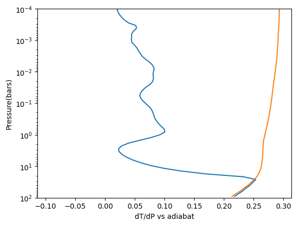
Check Adiabat
This plot and datareturn is helpful to check that there have been no issues with where the code has found the location of the convective zone(s). See below, dTdP never exceeds the adiabat.
[12]:
adiabat, dtdp, pressure = jpi.pt_adiabat(out, cl_run)