Using Correlated-K Tables vs. Monochromatic Opacities
Throughout the tutorials, we have always used monochromatic opacities. If you are interested in switching to correlated-K tables versus using the currently provided opacities on Zenodo, that is possible. Here you will learn:
Running forward model with pre-weighted tables vs resort rebin vs resampled monochromatic opacities
Before completing this notebook you will have to:
Download at least one or multiple of the k-table folder File should be of the format
sonora_2121grid_feh+XXX_co_YYY, where XXX defines the Fe/H and YYY describes the C/O ratioDownload Sonora PT profiles (if this is unfamiliar please see Brown Dwarf Tutorial)
Download PICASO Correlated-K’s for On-the-Fly Disequilibrium Climate Calculations (see Brown Dwarf Tutorial)
These are all easily retrieved through the data.get_data function:
import picaso.data as d
d.get_data(category_download=’sonora_grids’,target_download=’bobcat’)
d.get_data(category_download=’ck_tables’,target_download=’pre-weighted’)
d.get_data(category_download=’ck_tables’,target_download=’by-molecule’)
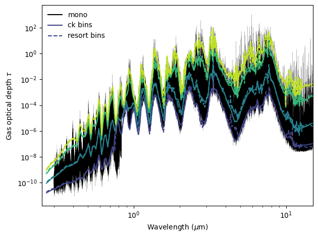
Compare the optical depth for various layers
One big difference you will notice between taugas for a monochromatic opacity calculation and a correlated-k calculation, is that taugas will have an extra dimension for CK. Those correspond to each of the gauss points. Now, be careful not to confuse the gauss points that we use for the disk integration and these gauss points. They are different!
Below is an example of summing the tau’s in order to compare with the monochromatic opacities.
This compares the mono case, the premixed correlated-k case, and the disequilibrium chemistry correlated-k case
[7]:
cm1_to_micron = lambda wn: 1e4 / wn

# Num gauss points is based on the opacities that you're using
num_gauss_points = 8
gauss_to_plot    = range(0, num_gauss_points, 2)
cmap             = plt.cm.viridis
colors           = cmap(np.linspace(0.2, 0.9, len(gauss_to_plot)))

wl_mono  = cm1_to_micron(df['mono']['wavenumber'])
wl_ck    = cm1_to_micron(df['ck']['wavenumber'])
wl_resort = cm1_to_micron(df['resort']['wavenumber'])

fig, ax = plt.subplots()

ax.plot(wl_mono,
        df['mono']['full_output']['taugas'][0],
        color='black', lw=0.1, alpha=1, label='mono')

# CK = solid, resort = dashed; color varies per Gauss index
for j, i in enumerate(gauss_to_plot):
    clr = colors[j]
    ax.plot(wl_ck,    df['ck']['full_output']['taugas'][0, :, i], lw=1.5, ls='-', color=clr)
    ax.plot(wl_resort, df['resort']['full_output']['taugas'][0, :, i], lw=1.5, ls='--', color=clr)

# axes formatting
ax.set(xscale='log', yscale='log',
       xlim=(0.25, 15),
       xlabel=r'Wavelength ($\mu$m)',
       ylabel=r'Gas optical depth $\tau$')

# legend with uniform linewidth
leg_lw = 1.5
legend_handles = [
    Line2D([], [], color='black',  lw=leg_lw, ls='-',  label='mono'),
    Line2D([], [], color=colors[0], lw=leg_lw, ls='-',  label='ck bins'),
    Line2D([], [], color=colors[0], lw=leg_lw, ls='--', label='resort bins'),
]
ax.legend(handles=legend_handles, frameon=False)

plt.tight_layout()
plt.show()
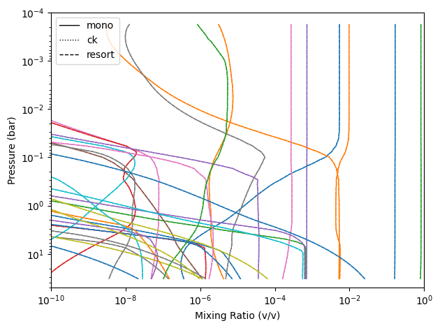
Compare Chemistry
In this case we supplied it the same chemistry. However, there may be cases where you want to extract the chemistry from the pre-computed files. This is how you would go about doing so.
For the below code snippet, I am pulling out the abundances that are higher than 0.1 ppm.
[8]:
styles = {'mono': '-', 'ck': ':', 'resort': '--'}
colors = cycle(plt.cm.tab10.colors)

fig, ax = plt.subplots()
ax.set(xscale='log', yscale='log', xlim=(1e-10, 1), ylim=(50, 1e-4), xlabel='Mixing Ratio (v/v)', ylabel='Pressure (bar)')

species = {c for k in styles for c in cases[k].inputs['atmosphere']['profile'].columns if c not in ('pressure', 'temperature')}

for clr, sp in zip(colors, species):
    for case, ls in styles.items():
        df = cases[case].inputs['atmosphere']['profile']
        x = df.get(sp)
        if x is not None and x.max() > 1e-8:
            ax.plot(x, df['pressure'], color=clr, ls=ls, lw=1)

ax.legend([Line2D([], [], color='k', lw=1, ls=ls) for ls in styles.values()], styles.keys())
plt.tight_layout()