Note

Download full notebook here

Brown Dwarf Models

Modeling brown dwarfs is very similar to modeling thermal emission for exoplanets. The only difference is there is no stellar input!

In this tutorial you will learn:

1. How to turn that feature off

2. Query a profile from the Sonora Grid. Note, this is note necessary – just convenient!

3. Create a Brown Dwarf Spectrum

import warnings
warnings.filterwarnings('ignore')
import numpy as np
import pandas as pd
import astropy.units as u

#picaso
from picaso import justdoit as jdi
from picaso import justplotit as jpi
#plotting
from bokeh.io import output_notebook

output_notebook()
from bokeh.plotting import show,figure

Loading BokehJS ...

Start with the same inputs as before

wave_range = [3,5]

opa = jdi.opannection(wave_range=wave_range)

bd = jdi.inputs(calculation='browndwarf')

# Note here that we do not need to provide case.star, since there is none!
bd.gravity(gravity=100 , gravity_unit=u.Unit('m/s**2'))

#this is the integration setup that was used to compute the Sonora grid
#take a look at Spherical Integration Tutorial to get a look at what these parameters do
bd.phase_angle(0)

Download and Query from Sonora Profile Grid

Download the profile files that are located in the profile.tar file

Once you untar the file you can set the file path below. You do not need to unzip each profile. picaso will do that upon read in. picaso will find the nearest neighbor and attach it to your class.

#point to where you untared your sonora profiles
sonora_profile_db = '/data/sonora_profile/'
Teff = 900
#this function will grab the gravity you have input above and find the nearest neighbor with the
#note sonora chemistry grid is on the same opacity grid as our opacities (1060).
bd.sonora(sonora_profile_db, Teff)

Note if you have added anything to your atmosphere profile (bd.inputs['atmosphere']['profile']), sonora function will overwrite it! Therefore, make sure that you add new column fields after running sonora.

Run Spectrum

df = bd.spectrum(opa, full_output=True)

Convert to \(F_\nu\) Units and Regrid

PICASO outputs the raw flux as:

\[F_\lambda ( \frac{erc}{cm^2 * sec * cm})\]

Typical fluxes shown in several Brown Dwarf papers are:

\[F_\nu ( \frac{erc}{cm^2 * sec * Hz})\]

Below is a little example of how to convert units.

NOTE: Some people like to plot out Eddington Flux, \(H_\nu\). This gets confusing as the units appear to be erg/cm2/s/Hz but you will notice a factor of four difference:

\[H_\nu = \frac{F_\nu}{4}\]

x,y = df['wavenumber'], df['thermal'] #units of erg/cm2/s/cm

xmicron = 1e4/x

flamy = y*1e-8 #per anstrom instead of per cm
sp = jdi.psyn.ArraySpectrum(xmicron, flamy,
                            waveunits='um',
                            fluxunits='FLAM')
sp.convert("um")
sp.convert('Fnu') #erg/cm2/s/Hz

x = sp.wave #micron
y= sp.flux #erg/cm2/s/Hz
df['fluxnu'] = y
x,y = jdi.mean_regrid(1e4/x, y, R=300) #wavenumber, erg/cm2/s/Hz
df['regridy'] =  y
df['regridx'] = x

Compare with Sonora Grid

The corresponding spectra are also available at the same link above. PICASO doesn’t provide query functions for this. So if you want to compare, you will have to read in the files as is done below

son = pd.read_csv('sp_t900g100nc_m0.0',delim_whitespace=True,
                 skiprows=3,header=None,names=['w','f'])
sonx, sony =  jdi.mean_regrid(1e4/son['w'], son['f'], newx=x)

show(jpi.spectrum([x]*2,[df['regridy'], sony], legend=['PICASO', 'Sonora']
                  ,plot_width=800,x_range=wave_range,y_axis_type='log'))

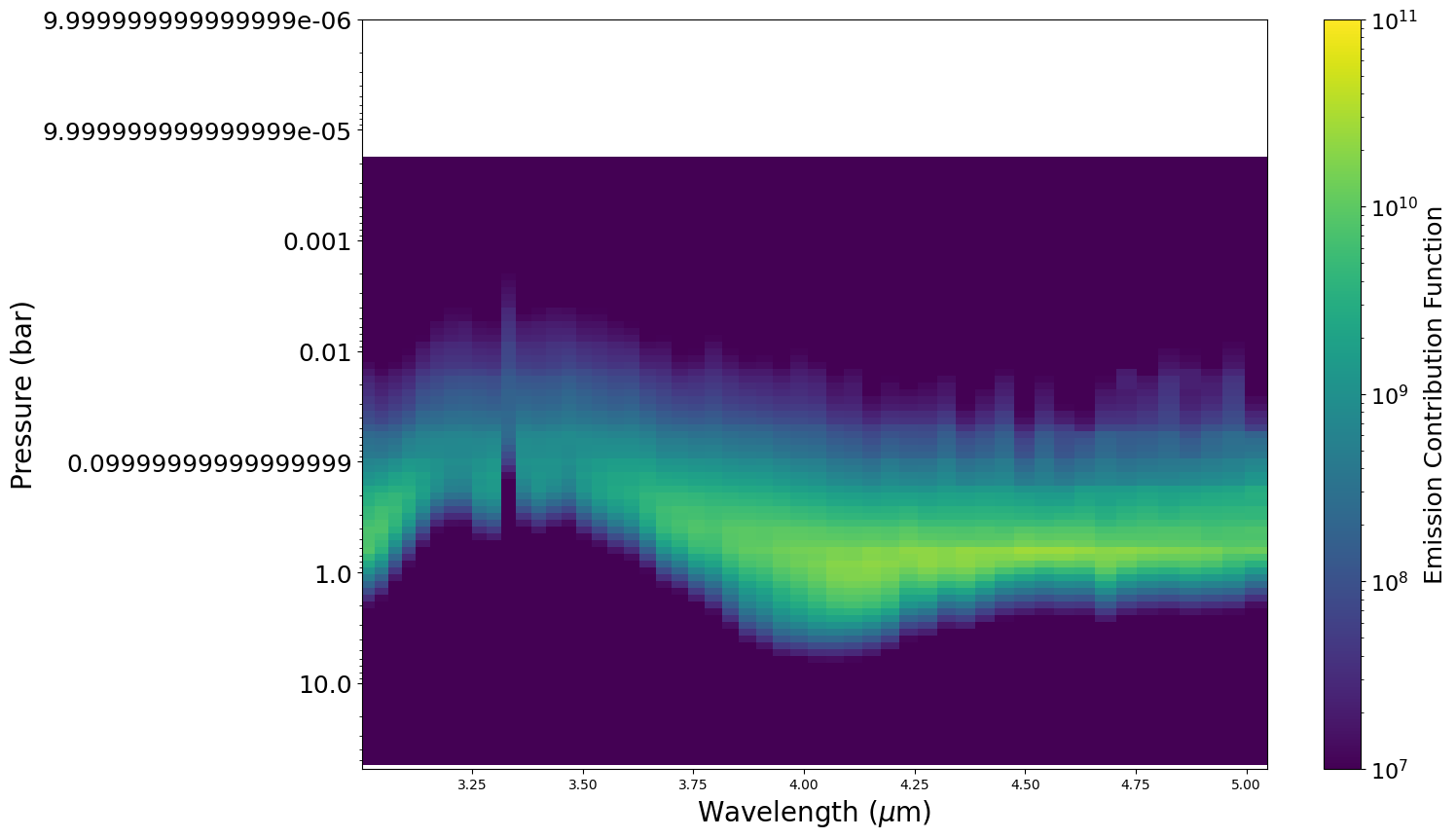
Thermal Contribution Function

Contribution functions give us an understanding of where pressures flux is being emitted (e.g. Lothringer et al 2018 Figure 12)

fig, ax, CF = jpi.thermal_contribution(df['full_output'], norm=jpi.colors.LogNorm(vmin=1e7, vmax=1e11))