One-Dimensional Climate Models: The Basics of Planets
In this tutorial you will learn the very basics of running 1D climate runs. For a more in depth look at the climate code check out Mukherjee et al. 2023 (note this should also be cited if using this code/tutorial).
What you should already be familiar with:
What you will need to download to use this tutorial:
Download New 1460 PT, 196 wno Correlated-k Tables to be used by the climate code for opacity (if you completed the brown dwarf tutorial you should already have this)
Download the PHOENIX stellar models.
You can easily do this with the get_data function
import picaso.data as d
d.get_data(category_download=’ck_tables’,target_download=’by-molecule’)
d.get_data(category_download=’stellar_grids’,target_download=’phoenix’)
Note: the two files above are dependent on metallicity and C/O.
[1]:
import os
import warnings
warnings.filterwarnings('ignore')
import picaso.justdoit as jdi
import picaso.justplotit as jpi
import astropy.units as u
import numpy as np
import matplotlib.pyplot as plt
%matplotlib inline
[2]:
#1 ck tables from roxana
mh = '1.0'#'+1.0' #log metallicity, 10xSolar
CtoO = '0.46'#'1.0' # CtoO ratio, Solar C/O

ck_db = os.path.join(os.getenv('picaso_refdata'),'opacities', 'preweighted', f'sonora_2121grid_feh{mh}_co{CtoO}.hdf5')
[3]:
# Notice The keyword ck is set to True because you want to use the correlated-k opacities for your calculation
# and not the line by line opacities
opacity_ck = jdi.opannection(ck_db=ck_db,method='preweighted') # grab your opacities
Starting up the Run
You will notice that starting a run is nearly identical as running a spectrum and brown dwarf climate model. However, how we will add climate=True to our inputs flag. We will also specify planet in this case, which will turn on the irradiation the object is receiving.
New Parameter (was also used in the Brown Dwarf tutorial): Effective Temperature. This excerpt from Modeling Exoplanetary Atmospheres (Fortney et al) provides a thorough description and more reading, if you are interested.
If the effective temperature, \(T_{eff}\), is defined as the temperature of a blackbody of the same radius that would emit the equivalent flux as the real planet, \(T_{eff}\) and \(T_{eq}\) can be simply related. This relation requires the inclusion of a third temperature, \(T_{int}\), the intrinsic effective temperature, that describes the flux from the planet’s interior. These temperatures are related by:
\(T_{eff}^4 = T_{int}^4 + T_{eq}^4\)
We then recover our limiting cases: if a planet is self-luminous (like a young giant planet) and far from its parent star, \(T_{eff} \approx T_{int}\); for most rocky planets, or any planets under extreme stellar irradiation, \(T_{eff} \approx T_{eq}\).
[4]:
cl_run = jdi.inputs(calculation="planet", climate = True) # start a calculation

#note you need to put the climate keyword to be True in order to do so
# now you need to add these parameters to your calculation


tint= 200 # Intrinsic Temperature of your Planet in K
grav = 4.5 # Gravity of your Planet in m/s/s

cl_run.gravity(gravity=grav, gravity_unit=u.Unit('m/(s**2)')) # input gravity
cl_run.effective_temp(tint) # input effective temperature
Let’s now input the host-star properties
[5]:
T_star =5326.6 # K, star effective temperature
logg =4.38933 #logg , cgs
metal =-0.03 # metallicity of star
r_star = 0.932 # solar radius
semi_major = 0.0486 # star planet distance, AU

cl_run.star(opacity_ck, temp =T_star,metal =metal, logg =logg, radius = r_star,database='phoenix',
            radius_unit=u.R_sun,semi_major= semi_major , semi_major_unit = u.AU)
Initial T(P) Guess
Every calculation requires an initial guess of the pressure temperature profile. The code will iterate from there to find the correct solution. A few tips:
We recommend using typically 51-91 atmospheric pressure levels. Too many pressure layers increases the computational time required for convergence. Too little layers makes the atmospheric grid too coarse for an accurate calculation.
Start with a guess that is close to your expected solution. One easy way to get fairly close is by using the Guillot et al 2010 temperature-pressure profile approximation
[6]:
nlevel = 91 # number of plane-parallel levels in your code

#Lets set the max and min at 1e-4 bars and 500 bars
Teq=1000 # planet equilibrium temperature
pt = cl_run.guillot_pt(Teq, nlevel=nlevel, T_int = tint, p_bottom=2, p_top=-6)
temp_guess = pt['temperature'].values
pressure = pt['pressure'].values
Initial Convective Zone Guess
You also need to have a crude guess of the convective zone of your atmosphere. Generally the deeper atmosphere is always convective. Again a good guess is always the published SONORA grid of models for this. But lets assume that the bottom 7 levels of the atmosphere is convective.
New Parameters:
rfacv: (See Mukherjee et al. 2023 Eqn. 20r_st)
Non-zero values of rst (aka “rfacv” legacy terminology) is only relevant when the external irradiation on the atmosphere is non-zero. In the scenario when a user is computing a planet-wide average T(P) profile, the stellar irradiation is contributing to 50% (one hemisphere) of the planet and as a result rst = 0.5. If instead the goal is to compute a night-side average atmospheric state, rst is set to be 0. On the other extreme, to compute the day-side atmospheric state of a tidally locked planet rst should be set at 1.
[7]:
rcb_guess = 85 # top most level of guessed convective zone

# Here are some other parameters needed for the code.
rfacv = 0.5 #we are focused on a brown dwarf so let's keep this as is
Now we would use the inputs_climate function to input everything together to our cl_run we started.
[8]:
cl_run.inputs_climate(temp_guess= temp_guess, pressure= pressure,
                      rcb_guess=rcb_guess, rfacv = rfacv)
Run the Climate Code
The actual climate code can be run with the cl_run.run command. The save_all_profiles is set to True to save the T(P) profile at all steps. The code will now iterate from your guess to reach the correct atmospheric solution for your brown dwarf of interest.
[9]:
out = cl_run.climate(opacity_ck, save_all_profiles=True,with_spec=True)
SUMMARY
-------
Clouds: False
quench False
cold_trap False
vol_rainout False
no_ph3 False
Moist Adiabat: False
Iteration number  0 , min , max temp  857.891950050302 2293.489765369266 , flux balance  0.24586805323301847
Iteration number  1 , min , max temp  825.5532298480927 2768.9875908947215 , flux balance  15.468720921315139
Iteration number  2 , min , max temp  823.463745745593 2648.9650134030294 , flux balance  0.2722544197601914
Iteration number  3 , min , max temp  823.4446145455615 2635.5916060601194 , flux balance  0.0014843772530978212
Iteration number  4 , min , max temp  823.4445103063792 2635.404319771508 , flux balance  7.539558433178064e-06
In t_start: Converged Solution in iterations  4
Big iteration is  823.4445103063792 0
 We are already at a root, tolf , test =  5e-05 ,  1.1417209376238072e-05
Profile converged before itmx
Iteration number  0 , min , max temp  819.7214913162957 2726.6998607756836 , flux balance  1.1003740239657238
Iteration number  1 , min , max temp  814.7326382540977 2817.7498481275484 , flux balance  0.19705910074854008
Iteration number  2 , min , max temp  814.6622197922778 2812.6537509788036 , flux balance  0.0011923310664987655
In t_start: Converged Solution in iterations  2
Big iteration is  814.6622197922778 0
Iteration number  0 , min , max temp  814.6618396151556 2812.625425336018 , flux balance  6.500053131255152e-06
In t_start: Converged Solution in iterations  0
Profile converged before itmx
Iteration number  0 , min , max temp  809.5097543297865 2830.5744748896304 , flux balance  0.016850644665374438
Iteration number  1 , min , max temp  809.4356579198734 2828.883009091387 , flux balance  0.00010682290897799364
In t_start: Converged Solution in iterations  1
Big iteration is  809.4356579198734 0
Iteration number  0 , min , max temp  809.4352624844934 2828.877031509815 , flux balance  6.312766194081936e-07
In t_start: Converged Solution in iterations  0
Profile converged before itmx
Iteration number  0 , min , max temp  807.6049245392105 2811.4052984988853 , flux balance  0.0012432801842257157
In t_start: Converged Solution in iterations  0
Big iteration is  807.6049245392105 0
Iteration number  0 , min , max temp  807.5893131192433 2811.394403395632 , flux balance  8.215615786276766e-06
In t_start: Converged Solution in iterations  0
Profile converged before itmx
final [0, 83, 89, 0, 0, 0]
Iteration number  0 , min , max temp  807.6827329802513 2812.520240725085 , flux balance  0.0002390937769113331
In t_start: Converged Solution in iterations  0
Big iteration is  807.6827329802513 0
Iteration number  0 , min , max temp  807.6831742227286 2812.5223251233124 , flux balance  1.3892854960271714e-06
In t_start: Converged Solution in iterations  0
Profile converged before itmx
YAY ! ENDING WITH CONVERGENCE
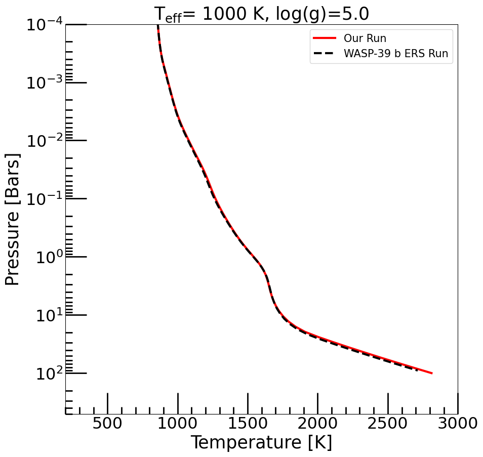
[10]:
base_case = jdi.pd.read_csv(jdi.HJ_pt(), sep=r'\s+')

plt.figure(figsize=(10,10))
plt.ylabel("Pressure [Bars]", fontsize=25)
plt.xlabel('Temperature [K]', fontsize=25)
plt.ylim(500,1e-4)
plt.xlim(200,3000)

plt.semilogy(out['temperature'],out['pressure'],color="r",linewidth=3,label="Our Run")

plt.semilogy(base_case['temperature'],base_case['pressure'],color="k",linestyle="--",linewidth=3,label="WASP-39 b ERS Run")


plt.minorticks_on()
plt.tick_params(axis='both',which='major',length =30, width=2,direction='in',labelsize=23)
plt.tick_params(axis='both',which='minor',length =10, width=2,direction='in',labelsize=23)

plt.legend(fontsize=15)

plt.title(r"T$_{\rm eff}$= 1000 K, log(g)=5.0",fontsize=25)
[10]:
Text(0.5, 1.0, 'T$_{\\rm eff}$= 1000 K, log(g)=5.0')
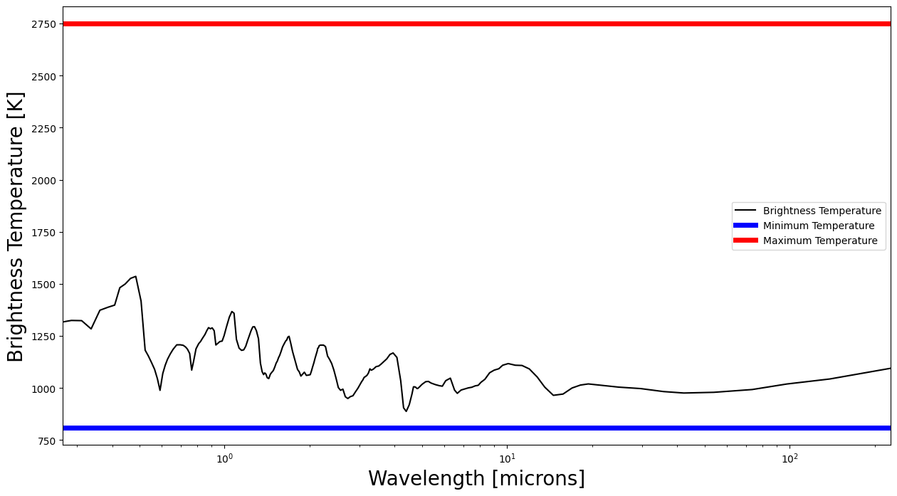
Brightness Temperature
Checking the brightness temperature serves many useful purposes:
Intuition building. Allows you to see what corresponding temperature are you sensitive to at each wavelength
Note that this temperature doesn’t need to be the physical temperature of your atmosphere but if you can find the physical converged atmospheric temperature closest to this brightness temperature you can also get an idea of the atmospheric pressure from where the flux you are seeing is originating from.
Determining if your choice in bottom boundary pressure grid was correct.
If your brightness temperature is such that you bottom out at the temperature corresponding to the highest pressure, you have not extended your grid to high enough pressures.
Brightness Temperature Equation:
\(T_{\rm bright}=\dfrac{a}{{\lambda}log\left(\dfrac{{b}}{F(\lambda){\lambda}^5}+1\right)}\)
where a = 1.43877735$:nbsphinx-math:times\(10\)^{-2}$ m.K and b = 11.91042952$:nbsphinx-math:times\(10\)^{-17}$ m\(^4\)kg/s\(^3\)
Let’s calculate the brightness temperature of our current run and check if our pressure grid was okay.
[11]:
brightness_temp, figure= jpi.brightness_temperature(out['spectrum_output'])
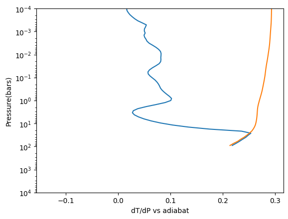
Check Adiabat
This plot and datareturn is helpful to check that there have been no issues with where the code has found the location of the convective zone(s). See below, dTdP never exceeds the adiabat.
[12]:
import importlib;importlib.reload(jpi)
[12]:
<module 'picaso.justplotit' from '/home/nbatalh1/codes/picaso/picaso/justplotit.py'>
[13]:
cp, adiabat, dtdp, pressure = jpi.pt_adiabat(out, cl_run, opacity_ck, plot=True)
[14]:
jdi.output_xarray(out,cl_run,savefile='w39.nc')
[14]:
<xarray.Dataset> Size: 59kB
Dimensions:         (pressure: 91, pressure_layer: 90, wavelength: 196)
Coordinates:
  * pressure        (pressure) float64 728B 1e-06 1.227e-06 ... 81.49 100.0
  * pressure_layer  (pressure_layer) float64 720B 1.108e-06 1.359e-06 ... 90.27
  * wavelength      (wavelength) float64 2kB 227.5 138.8 97.75 ... 0.287 0.2679
Data variables: (12/76)
    temperature     (pressure) float64 728B 857.0 833.6 ... 2.69e+03 2.813e+03
    dtdp            (pressure_layer) float64 720B -0.1351 -0.06234 ... 0.2181
    guess 1         (pressure) float64 728B 861.5 861.5 ... 1.876e+03 1.933e+03
    guess 2         (pressure) float64 728B 861.5 861.5 ... 2.114e+03 2.226e+03
    guess 3         (pressure) float64 728B 861.5 861.5 ... 2.114e+03 2.226e+03
    guess 4         (pressure) float64 728B 861.5 859.6 ... 2.18e+03 2.293e+03
    ...              ...
    Mg+             (pressure) float64 728B 3.456e-41 4.021e-43 ... 2.753e-10
    Si              (pressure) float64 728B 6.984e-32 1.829e-33 ... 5.969e-07
    Fe+             (pressure) float64 728B 4.405e-39 7.155e-41 ... 6.194e-11
    Ti              (pressure) float64 728B 8.889e-35 1.975e-36 ... 8.604e-08
    Ti+             (pressure) float64 728B 1e-50 1e-50 ... 3.606e-13 1.151e-12
    C+              (pressure) float64 728B 1e-50 1e-50 ... 2.024e-25 3.293e-24
Attributes:
    climate_params:  {"cvs_locs": [0, 83, 89, 0, 0, 0], "converged": 1}
    planet_params:   {"effective_temp": 1087.1215242417622, "gravity": {"valu...
    stellar_params:  {"database": "phoenix", "steff": 5326.6, "feh": -0.03, "...
orbit_params: {"sma": {"value": 727045651602.0, "unit": "cm"}}- pressure: 91
- pressure_layer: 90
- wavelength: 196
- pressure(pressure)float641e-06 1.227e-06 ... 81.49 100.0
- units :
- bar
array([1.000000e-06, 1.227125e-06, 1.505836e-06, 1.847850e-06, 2.267543e-06, 2.782559e-06, 3.414549e-06, 4.190079e-06, 5.141752e-06, 6.309573e-06, 7.742637e-06, 9.501185e-06, 1.165914e-05, 1.430723e-05, 1.755676e-05, 2.154435e-05, 2.643761e-05, 3.244226e-05, 3.981072e-05, 4.885274e-05, 5.994843e-05, 7.356423e-05, 9.027252e-05, 1.107757e-04, 1.359356e-04, 1.668101e-04, 2.046968e-04, 2.511886e-04, 3.082399e-04, 3.782490e-04, 4.641589e-04, 5.695811e-04, 6.989473e-04, 8.576959e-04, 1.052500e-03, 1.291550e-03, 1.584893e-03, 1.944862e-03, 2.386590e-03, 2.928645e-03, 3.593814e-03, 4.410059e-03, 5.411695e-03, 6.640828e-03, 8.149127e-03, 1.000000e-02, 1.227125e-02, 1.505836e-02, 1.847850e-02, 2.267543e-02, 2.782559e-02, 3.414549e-02, 4.190079e-02, 5.141752e-02, 6.309573e-02, 7.742637e-02, 9.501185e-02, 1.165914e-01, 1.430723e-01, 1.755676e-01, 2.154435e-01, 2.643761e-01, 3.244226e-01, 3.981072e-01, 4.885274e-01, 5.994843e-01, 7.356423e-01, 9.027252e-01, 1.107757e+00, 1.359356e+00, 1.668101e+00, 2.046968e+00, 2.511886e+00, 3.082399e+00, 3.782490e+00, 4.641589e+00, 5.695811e+00, 6.989473e+00, 8.576959e+00, 1.052500e+01, 1.291550e+01, 1.584893e+01, 1.944862e+01, 2.386590e+01, 2.928645e+01, 3.593814e+01, 4.410059e+01, 5.411695e+01, 6.640828e+01, 8.149127e+01, 1.000000e+02]) - pressure_layer(pressure_layer)float641.108e-06 1.359e-06 ... 73.56 90.27
- units :
- bars
array([1.107757e-06, 1.359356e-06, 1.668101e-06, 2.046968e-06, 2.511886e-06, 3.082399e-06, 3.782490e-06, 4.641589e-06, 5.695811e-06, 6.989473e-06, 8.576959e-06, 1.052500e-05, 1.291550e-05, 1.584893e-05, 1.944862e-05, 2.386590e-05, 2.928645e-05, 3.593814e-05, 4.410059e-05, 5.411695e-05, 6.640828e-05, 8.149127e-05, 1.000000e-04, 1.227125e-04, 1.505836e-04, 1.847850e-04, 2.267543e-04, 2.782559e-04, 3.414549e-04, 4.190079e-04, 5.141752e-04, 6.309573e-04, 7.742637e-04, 9.501185e-04, 1.165914e-03, 1.430723e-03, 1.755676e-03, 2.154435e-03, 2.643761e-03, 3.244226e-03, 3.981072e-03, 4.885274e-03, 5.994843e-03, 7.356423e-03, 9.027252e-03, 1.107757e-02, 1.359356e-02, 1.668101e-02, 2.046968e-02, 2.511886e-02, 3.082399e-02, 3.782490e-02, 4.641589e-02, 5.695811e-02, 6.989473e-02, 8.576959e-02, 1.052500e-01, 1.291550e-01, 1.584893e-01, 1.944862e-01, 2.386590e-01, 2.928645e-01, 3.593814e-01, 4.410059e-01, 5.411695e-01, 6.640828e-01, 8.149127e-01, 1.000000e+00, 1.227125e+00, 1.505836e+00, 1.847850e+00, 2.267543e+00, 2.782559e+00, 3.414549e+00, 4.190079e+00, 5.141752e+00, 6.309573e+00, 7.742637e+00, 9.501185e+00, 1.165914e+01, 1.430723e+01, 1.755676e+01, 2.154435e+01, 2.643761e+01, 3.244226e+01, 3.981072e+01, 4.885274e+01, 5.994843e+01, 7.356423e+01, 9.027252e+01]) - wavelength(wavelength)float64227.5 138.8 97.75 ... 0.287 0.2679
- units :
- micron
array([227.531286, 138.792505,  97.751711,  73.691968,  53.87931 ,  42.211904,
        35.752592,  29.70003 ,  24.838549,  21.394951,  19.381723,  18.180165,
        16.977929,  15.776603,  14.575135,  13.58788 ,  12.786906,  11.986096,
        11.29178 ,  10.691757,  10.091327,   9.647853,   9.347542,   8.995233,
         8.673027,   8.345156,   8.074283,   7.903889,   7.713966,   7.498219,
         7.283852,   7.093708,   6.872616,   6.663779,   6.515295,   6.297428,
         6.063914,   5.899009,   5.759373,   5.572117,   5.379091,   5.264682,
         5.149065,   4.99975 ,   4.881621,   4.82742 ,   4.796393,   4.749804,
         4.699911,   4.662331,   4.605006,   4.504099,   4.395218,   4.300705,
         4.201857,   4.073652,   3.949369,   3.849337,   3.74932 ,   3.662132,
         3.587122,   3.513148,   3.43808 ,   3.36338 ,   3.307835,   3.269069,
         3.230939,   3.193434,   3.155918,   3.118422,   3.084777,   3.054764,
         3.014477,   2.964742,   2.908583,   2.846813,   2.787456,   2.730375,
         2.675585,   2.622951,   2.573572,   2.527199,   2.481605,   2.436796,
         2.394177,   2.353606,   2.314333,   2.276478,   2.240018,   2.208932,
         2.182822,   2.162525,   2.147732,   2.136535,   2.128826,   2.113562,
         2.091066,   2.069847,   2.049842,   2.029839,   2.009848,   1.982033,
         1.94705 ,   1.916269,   1.88935 ,   1.863065,   1.837391,   1.812317,
         1.788365,   1.765568,   1.740462,   1.713268,   1.691532,   1.674874,
         1.659751,   1.646091,   1.627432,   1.604029,   1.583694,   1.567152,
         1.552289,   1.537586,   1.522557,   1.506024,   1.488095,   1.470588,
         1.452433,   1.433692,   1.415929,   1.40007 ,   1.386482,   1.374098,
         1.35829 ,   1.339298,   1.318457,   1.295962,   1.276068,   1.25857 ,
         1.24106 ,   1.22356 ,   1.206051,   1.188555,   1.169211,   1.148221,
         1.125613,   1.101619,   1.080246,   1.06125 ,   1.039574,   1.015582,
         0.996011,   0.980416,   0.962798,   0.943913,   0.931485,   0.918911,
         0.903959,   0.891452,   0.877435,   0.865475,   0.852159,   0.834147,
         0.822341,   0.80973 ,   0.792428,   0.777427,   0.764968,   0.752426,
         0.738951,   0.728775,   0.714255,   0.696874,   0.677124,   0.657415,
         0.642413,   0.627973,   0.616515,   0.604407,   0.59094 ,   0.578428,
         0.565425,   0.551911,   0.536933,   0.523492,   0.506396,   0.484938,
         0.464786,   0.444776,   0.42581 ,   0.408323,   0.387097,   0.362069,
         0.337037,   0.312   ,   0.286957,   0.267868])
- temperature(pressure)float64857.0 833.6 ... 2.69e+03 2.813e+03
- units :
- Kelvin
array([ 856.96823291, 833.60315007, 823.0342704 , 815.03780946, 810.05952948, 807.87840499, 807.68317422, 808.82767322, 810.89538893, 813.61783668, 816.80476953, 820.28908894, 823.90508194, 827.58952979, 831.32078925, 835.05163216, 838.75691423, 842.42637503, 846.11910505, 849.61555148, 852.50527882, 855.18885071, 858.07070894, 860.92668343, 863.91645579, 867.34256946, 871.34766476, 876.14012895, 881.83976769, 888.65880133, 897.05681685, 907.02177417, 916.79498211, 926.2824559 , 935.8255892 , 945.78264711, 955.4232533 , 965.3731894 , 975.94411784, 987.04708059, 999.1389151 , 1012.77019787, 1027.90404183, 1044.3508201 , 1061.80858081, 1079.8132293 , 1098.08645515, 1116.58129312, 1135.44552288, 1154.50274562, 1173.1552517 , 1190.62207576, 1206.71037138, 1221.63268252, 1235.97708708, 1250.60950015, 1266.31863832, 1283.48658021, 1302.19180299, 1322.15690961, 1343.21710844, 1365.19702219, 1388.0495861 , 1412.18940958, 1437.99306514, 1465.69745104, 1495.48072303, 1527.07814443, 1558.89254721, 1587.84801842, 1611.49492525, 1629.20189639, 1641.77056375, 1651.54756827, 1660.80508258, 1671.38547909, 1684.70983646, 1701.85554427, 1724.10118471, 1752.98860408, 1790.78432197, 1840.76998868, 1908.01058123, 2002.4613122 , 2109.22075473, 2219.35169264, 2333.08288669, 2449.43643504, 2568.50244662, 2689.71336017, 2812.52232512]) - dtdp(pressure_layer)float64-0.1351 -0.06234 ... 0.2253 0.2181
- units :
- K/bar
array([-0.13506048, -0.06234106, -0.04770184, -0.02993423, -0.01317303, -0.00118084, 0.00691837, 0.01247433, 0.01637584, 0.0191003 , 0.02079754, 0.02149028, 0.02180032, 0.0219786 , 0.02187774, 0.02163132, 0.02132822, 0.02136989, 0.02014821, 0.01658952, 0.01535573, 0.01643678, 0.01623478, 0.01693775, 0.0193378 , 0.02250911, 0.02679863, 0.03168121, 0.03763537, 0.04595517, 0.05397482, 0.05236329, 0.05030112, 0.05007913, 0.05170978, 0.04955024, 0.05061855, 0.05320932, 0.05527032, 0.05949007, 0.06620669, 0.07246868, 0.07755568, 0.08099796, 0.08215215, 0.08198877, 0.0816054 , 0.08185449, 0.08132251, 0.07830584, 0.07220747, 0.06557754, 0.06004797, 0.05703499, 0.05750217, 0.06098935, 0.06579375, 0.07069078, 0.07434047, 0.07721118, 0.07930257, 0.08110855, 0.08423965, 0.08846822, 0.09323484, 0.09828548, 0.10215498, 0.10074284, 0.08991844, 0.07222512, 0.0533921 , 0.03754752, 0.0290095 , 0.02731026, 0.03102704, 0.03879548, 0.0494728 , 0.06345064, 0.08118385, 0.10422215, 0.13450772, 0.1752891 , 0.23606275, 0.2537764 , 0.24867104, 0.24417044, 0.23778006, 0.23190536, 0.22529268, 0.21813726]) - guess 1(pressure)float64861.5 861.5 ... 1.876e+03 1.933e+03
- units :
- Kelvin
array([ 861.50559322, 861.50995149, 861.51528491, 861.52180556, 861.52976982, 861.53974374, 861.55206343, 861.56718729, 861.58573965, 861.60847964, 861.63632896, 861.67040506, 861.71206038, 861.76292894, 861.82661785, 861.90526334, 862.00177716, 862.12012176, 862.26510754, 862.44256429, 862.65954402, 862.92455974, 863.24786546, 863.6520784 , 864.15037031, 864.76063637, 865.50710167, 866.41889036, 867.5308904 , 868.88472626, 870.52983922, 872.52467116, 874.99760455, 878.0156938 , 881.66852508, 886.07388204, 891.36540144, 897.69257793, 905.21998499, 914.12552248, 924.59750268, 937.05666634, 951.58355688, 968.2967209 , 987.34168951, 1008.82673799, 1032.81270529, 1059.30346194, 1088.23733361, 1119.47971525, 1153.00506591, 1188.24891155, 1224.71230517, 1261.87134352, 1299.11996583, 1335.77952214, 1371.11508149, 1404.36032956, 1434.75293099, 1461.10637807, 1483.10885318, 1500.65810965, 1513.8571051 , 1523.13106472, 1529.17675886, 1532.85734081, 1535.0609711 , 1536.55311334, 1537.89126027, 1539.4020979 , 1541.21180632, 1543.41160193, 1546.09019172, 1549.34740864, 1553.30051919, 1558.08763021, 1563.87056388, 1571.00492936, 1579.66678841, 1590.09103671, 1602.58431514, 1617.4882286 , 1635.17761979, 1656.05710083, 1680.55571497, 1709.1196826 , 1742.77778421, 1781.68555959, 1826.12322213, 1876.47616293, 1933.09121914]) - guess 2(pressure)float64861.5 861.5 ... 2.114e+03 2.226e+03
- units :
- Kelvin
array([ 861.50559322, 861.50995149, 861.51528491, 861.52180556, 861.52976982, 861.53974374, 861.55206343, 861.56718729, 861.58573965, 861.60847964, 861.63632896, 861.67040506, 861.71206038, 861.76292894, 861.82661785, 861.90526334, 862.00177716, 862.12012176, 862.26510754, 862.44256429, 862.65954402, 862.92455974, 863.24786546, 863.6520784 , 864.15037031, 864.76063637, 865.50710167, 866.41889036, 867.5308904 , 868.88472626, 870.52983922, 872.52467116, 874.99760455, 878.0156938 , 881.66852508, 886.07388204, 891.36540144, 897.69257793, 905.21998499, 914.12552248, 924.59750268, 937.05666634, 951.58355688, 968.2967209 , 987.34168951, 1008.82673799, 1032.81270529, 1059.30346194, 1088.23733361, 1119.47971525, 1153.00506591, 1188.24891155, 1224.71230517, 1261.87134352, 1299.11996583, 1335.77952214, 1371.11508149, 1404.36032956, 1434.75293099, 1461.10637807, 1483.10885318, 1500.65810965, 1513.8571051 , 1523.13106472, 1529.17675886, 1532.85734081, 1535.0609711 , 1536.55311334, 1537.89126027, 1539.4020979 , 1541.21180632, 1543.41160193, 1546.09019172, 1549.34740864, 1553.30051919, 1558.08763021, 1563.87056388, 1571.00492936, 1579.66678841, 1590.09103671, 1602.58431514, 1617.4882286 , 1635.17761979, 1656.05710083, 1680.55571497, 1709.1196826 , 1804.35078266, 1903.64057806, 2006.96742856, 2114.41178795, 2225.68793704]) - guess 3(pressure)float64861.5 861.5 ... 2.114e+03 2.226e+03
- units :
- Kelvin
array([ 861.50559322, 861.50995149, 861.51528491, 861.52180556, 861.52976982, 861.53974374, 861.55206343, 861.56718729, 861.58573965, 861.60847964, 861.63632896, 861.67040506, 861.71206038, 861.76292894, 861.82661785, 861.90526334, 862.00177716, 862.12012176, 862.26510754, 862.44256429, 862.65954402, 862.92455974, 863.24786546, 863.6520784 , 864.15037031, 864.76063637, 865.50710167, 866.41889036, 867.5308904 , 868.88472626, 870.52983922, 872.52467116, 874.99760455, 878.0156938 , 881.66852508, 886.07388204, 891.36540144, 897.69257793, 905.21998499, 914.12552248, 924.59750268, 937.05666634, 951.58355688, 968.2967209 , 987.34168951, 1008.82673799, 1032.81270529, 1059.30346194, 1088.23733361, 1119.47971525, 1153.00506591, 1188.24891155, 1224.71230517, 1261.87134352, 1299.11996583, 1335.77952214, 1371.11508149, 1404.36032956, 1434.75293099, 1461.10637807, 1483.10885318, 1500.65810965, 1513.8571051 , 1523.13106472, 1529.17675886, 1532.85734081, 1535.0609711 , 1536.55311334, 1537.89126027, 1539.4020979 , 1541.21180632, 1543.41160193, 1546.09019172, 1549.34740864, 1553.30051919, 1558.08763021, 1563.87056388, 1571.00492936, 1579.66678841, 1590.09103671, 1602.58431514, 1617.4882286 , 1635.17761979, 1656.05710083, 1680.55571497, 1709.1196826 , 1804.35078266, 1903.64057806, 2006.96742856, 2114.41178795, 2225.68793704]) - guess 4(pressure)float64861.5 859.6 ... 2.18e+03 2.293e+03
- units :
- Kelvin
array([ 861.5036923 , 859.57412374, 859.14592311, 858.74768906, 858.45316153, 858.22644741, 858.05904629, 857.94751812, 857.89195005, 857.89261546, 857.94905148, 858.05896643, 858.21791755, 858.42174236, 858.66786178, 858.95344367, 859.28173589, 859.66108448, 860.10319542, 860.61271996, 861.18545462, 861.81907663, 862.51809176, 863.27440014, 864.10823049, 865.06384684, 866.17486288, 867.47978585, 869.0034198 , 870.78252958, 872.87866242, 875.35338689, 878.32278502, 881.85532352, 886.01037419, 890.95236621, 896.87295786, 903.89613327, 912.07827088, 921.50683916, 932.41438458, 945.30301538, 960.05140548, 976.69279386, 995.55333239, 1016.52164194, 1039.65379117, 1065.14818211, 1092.93862673, 1122.77877735, 1154.70211767, 1188.20129825, 1222.8236396 , 1258.15448616, 1293.67574365, 1328.8182589 , 1362.94487751, 1395.3137714 , 1425.17677546, 1451.34494999, 1473.46639419, 1491.43804425, 1505.37108564, 1515.71219763, 1523.1507975 , 1528.52331423, 1532.65841197, 1536.24375978, 1539.75713327, 1543.47204613, 1547.41999761, 1551.5946593 , 1556.00329531, 1560.7029488 , 1565.83668461, 1571.6173975 , 1578.35856494, 1586.59251377, 1596.6884191 , 1609.03404671, 1624.19098531, 1642.80561185, 1665.53047525, 1693.03228123, 1725.98445732, 1765.29915712, 1862.95453316, 1964.6004695 , 2070.3519031 , 2179.97336773, 2293.48976537]) - guess 5(pressure)float64861.5 842.8 ... 2.646e+03 2.769e+03
- units :
- Kelvin
array([ 861.47676157, 842.82730309, 838.62042565, 834.68432858, 831.7385264 , 829.43288498, 827.68422634, 826.4568853 , 825.7476143 , 825.55322985, 825.86132073, 826.63930577, 827.8310787 , 829.38059412, 831.22995233, 833.33180741, 835.69145026, 838.35450115, 841.39140169, 844.79456909, 848.45996483, 852.28985005, 856.2381216 , 860.03143446, 863.75203989, 867.67130513, 871.90256768, 876.5632346 , 881.59039576, 886.97840889, 892.89057736, 899.41321765, 906.5570758 , 914.40134318, 922.75178168, 932.16202257, 943.3033098 , 956.0821938 , 969.66034155, 983.39154045, 997.8806358 , 1014.30106213, 1030.88303506, 1046.96217133, 1064.33857394, 1081.08854255, 1097.19971117, 1114.44881655, 1132.71024599, 1150.76828192, 1169.10932871, 1187.67226436, 1206.37033381, 1225.72127417, 1245.99114333, 1267.61422701, 1290.8774452 , 1315.31707095, 1340.35895365, 1364.8284287 , 1388.03224874, 1409.86121978, 1430.48220345, 1450.49559419, 1470.46166846, 1490.89754974, 1512.01949324, 1533.76022941, 1555.86053722, 1578.12070931, 1599.78819647, 1620.09649281, 1638.46074018, 1654.67365795, 1669.15317572, 1682.75095747, 1696.99369901, 1713.79094451, 1734.97712316, 1762.04544547, 1797.3728809 , 1843.64217613, 1903.09324721, 1977.59182359, 2068.60812116, 2178.9817232 , 2291.49652868, 2407.1066448 , 2525.39154694, 2646.40908741, 2768.98759089]) - guess 6(pressure)float64861.4 842.2 ... 2.527e+03 2.649e+03
- units :
- Kelvin
array([ 861.41609505, 842.22613849, 837.75558424, 833.52269938, 830.3173101 , 827.78489593, 825.84919849, 824.48168067, 823.68622608, 823.46374575, 823.8017329 , 824.66240398, 825.97982404, 827.68699957, 829.71472115, 832.00623818, 834.5624884 , 837.42713704, 840.66821236, 844.26820823, 848.10870747, 852.0819492 , 856.13730961, 859.99570772, 863.74679556, 867.66636626, 871.86537584, 876.45602091, 881.37223253, 886.6072274 , 892.31801349, 898.58524376, 905.42255322, 912.90630158, 920.86358347, 929.81217553, 940.36635247, 952.44360044, 965.3162747 , 978.46565724, 992.4678522 , 1008.41100677, 1024.77563009, 1041.000009 , 1058.65893376, 1076.05957669, 1093.1243309 , 1111.35473704, 1130.55947569, 1149.48470842, 1168.41082637, 1187.07211665, 1205.18969399, 1223.17185907, 1241.33108773, 1260.35399695, 1280.95911601, 1303.09033116, 1326.52485022, 1350.34546432, 1373.90944244, 1397.11196698, 1419.99043791, 1442.89228317, 1465.92238558, 1489.07106027, 1512.08031457, 1534.60495884, 1556.34661857, 1577.23492956, 1596.78065604, 1614.56536423, 1630.35256212, 1644.19961142, 1656.62178447, 1668.42278563, 1680.88904282, 1695.59902816, 1713.98034624, 1737.16045028, 1766.92553558, 1805.19700787, 1853.44582063, 1912.86729524, 1984.46246195, 2070.27335017, 2179.434155 , 2292.22745335, 2408.28047576, 2527.16575292, 2648.9650134 ]) - guess 7(pressure)float64861.4 842.2 ... 2.514e+03 2.636e+03
- units :
- Kelvin
array([ 861.41517559, 842.22196776, 837.74941759, 833.51398453, 830.30606756, 827.77121488, 825.83333766, 824.4640789 , 823.66749614, 823.44461455, 823.78295039, 824.64463792, 825.96357471, 827.67257859, 829.70226023, 831.99573362, 834.55387233, 837.42030923, 840.6630415 , 844.26448644, 848.10615008, 852.08025229, 856.13619122, 859.99489204, 863.74607194, 867.66556135, 871.86430754, 876.45447478, 881.36994958, 886.60390004, 892.31324807, 898.57853279, 905.41330279, 912.89377192, 920.84707917, 929.79051025, 940.33745944, 952.40510236, 965.26704393, 978.40691957, 992.40087064, 1008.33585926, 1024.69717755, 1040.92502959, 1058.58981787, 1076.00188087, 1093.08090466, 1111.32352488, 1130.53753516, 1149.46889165, 1168.39731366, 1187.05704192, 1205.16774031, 1223.13283476, 1241.25630452, 1260.2173062 , 1280.73713298, 1302.77509387, 1326.13281544, 1349.91866214, 1373.50183759, 1396.77617323, 1419.75983171, 1442.77044788, 1465.88322488, 1489.07665115, 1512.10104596, 1534.6274031 , 1556.3666416 , 1577.24608643, 1596.76780022, 1614.50703197, 1630.2290418 , 1643.99988425, 1656.34336946, 1668.06658962, 1680.44813727, 1695.0490441 , 1713.26739543, 1736.19132527, 1765.53944376, 1803.11891076, 1850.21921855, 1907.79537558, 1976.58747128, 2058.29049072, 2167.074398 , 2279.48020706, 2395.27523175, 2513.89252195, 2635.59160606]) - guess 8(pressure)float64861.4 842.2 ... 2.514e+03 2.635e+03
- units :
- Kelvin
array([ 861.41516746, 842.22194342, 837.74938303, 833.51393683, 830.30600655, 827.77114083, 825.83325178, 824.46398342, 823.66739431, 823.44451031, 823.78284784, 824.64454071, 825.96348558, 827.67249921, 829.7021913 , 831.99567508, 834.55382378, 837.4202701 , 840.66301105, 844.26446352, 848.10613314, 852.08023969, 856.13618143, 859.99488356, 863.74606359, 867.66555217, 871.86429653, 876.45446083, 881.36993137, 886.603876 , 892.31321633, 898.57849102, 905.41324832, 912.89370152, 920.84698979, 929.79039676, 940.33731336, 952.40491437, 965.2668103 , 978.40664686, 992.40056552, 1008.33552391, 1024.69683229, 1040.9247005 , 1058.58951384, 1076.00162139, 1093.08069841, 1111.32336288, 1130.53740494, 1149.46877911, 1168.39720163, 1187.05691185, 1205.16756523, 1223.13256468, 1241.25584974, 1260.21653555, 1280.73591332, 1302.77335741, 1326.13062767, 1349.9162588 , 1373.49955546, 1396.77434419, 1419.75864676, 1442.76989749, 1465.88313199, 1489.07679382, 1512.10126193, 1534.62761981, 1556.36683692, 1577.24623046, 1596.76782447, 1614.50683826, 1630.22853552, 1643.99900534, 1656.34209528, 1668.06491414, 1680.44601359, 1695.04632571, 1713.26374658, 1736.18610909, 1765.53144445, 1803.10566971, 1850.1954774 , 1907.75024097, 1976.50016447, 2058.1227415 , 2166.90136222, 2279.30173644, 2395.09313403, 2513.70665788, 2635.40431977]) - guess 9(pressure)float64861.4 842.2 ... 2.514e+03 2.635e+03
- units :
- Kelvin
array([ 861.41516746, 842.22194342, 837.74938303, 833.51393683, 830.30600655, 827.77114083, 825.83325178, 824.46398342, 823.66739431, 823.44451031, 823.78284784, 824.64454071, 825.96348558, 827.67249921, 829.7021913 , 831.99567508, 834.55382378, 837.4202701 , 840.66301105, 844.26446352, 848.10613314, 852.08023969, 856.13618143, 859.99488356, 863.74606359, 867.66555217, 871.86429653, 876.45446083, 881.36993137, 886.603876 , 892.31321633, 898.57849102, 905.41324832, 912.89370152, 920.84698979, 929.79039676, 940.33731336, 952.40491437, 965.2668103 , 978.40664686, 992.40056552, 1008.33552391, 1024.69683229, 1040.9247005 , 1058.58951384, 1076.00162139, 1093.08069841, 1111.32336288, 1130.53740494, 1149.46877911, 1168.39720163, 1187.05691185, 1205.16756523, 1223.13256468, 1241.25584974, 1260.21653555, 1280.73591332, 1302.77335741, 1326.13062767, 1349.9162588 , 1373.49955546, 1396.77434419, 1419.75864676, 1442.76989749, 1465.88313199, 1489.07679382, 1512.10126193, 1534.62761981, 1556.36683692, 1577.24623046, 1596.76782447, 1614.50683826, 1630.22853552, 1643.99900534, 1656.34209528, 1668.06491414, 1680.44601359, 1695.04632571, 1713.26374658, 1736.18610909, 1765.53144445, 1803.10566971, 1850.1954774 , 1907.75024097, 1976.50016447, 2058.1227415 , 2166.90136222, 2279.30173644, 2395.09313403, 2513.70665788, 2635.40431977]) - guess 10(pressure)float64861.0 841.0 ... 2.604e+03 2.727e+03
- units :
- Kelvin
array([ 860.9565067 , 841.00184591, 835.3398847 , 830.27400803, 826.39893013, 823.47428112, 821.42282261, 820.18826096, 819.72149132, 819.96677953, 820.86252714, 822.32758851, 824.2511984 , 826.55124217, 829.15969844, 832.0116115 , 835.08934495, 838.40443596, 842.00389861, 845.86995082, 849.89662889, 853.518824 , 856.9140917 , 860.20728706, 863.54227115, 867.21962273, 871.35362979, 876.08549959, 881.40485493, 887.35208741, 894.06744712, 901.60519872, 909.79552119, 918.38782875, 927.2295283 , 936.7530296 , 947.46073283, 958.78345298, 970.31760009, 982.16517169, 995.00585011, 1009.82703772, 1025.64707455, 1042.02069587, 1059.64786965, 1077.37733192, 1095.06107551, 1113.40994301, 1132.42115849, 1151.37627871, 1170.16495853, 1188.30711173, 1205.58797926, 1222.31747161, 1238.95646007, 1256.27568851, 1275.01582636, 1295.28698219, 1317.07359231, 1339.68857631, 1362.56435465, 1385.5629305 , 1408.69828854, 1432.36106003, 1456.64495006, 1481.62776593, 1507.22552628, 1533.10148974, 1558.30675124, 1581.95759225, 1602.98551001, 1620.93107385, 1635.80360692, 1648.19612972, 1659.31958302, 1670.53381965, 1683.27618628, 1698.92064185, 1718.70732026, 1743.92530838, 1776.4841382 , 1818.33810934, 1871.94538273, 1939.99798649, 2026.91156683, 2140.24427873, 2251.57720501, 2366.45147341, 2483.96546589, 2604.37157478, 2726.69986078]) - guess 11(pressure)float64860.4 839.5 ... 2.695e+03 2.818e+03
- units :
- Kelvin
array([ 860.3853203 , 839.47832796, 832.31649994, 826.19335018, 821.46272506, 818.03516386, 815.83609476, 814.7747087 , 814.73263825, 815.57920811, 817.18776775, 819.4203399 , 822.10873531, 825.15201621, 828.48415545, 832.03048088, 835.75096047, 839.61845031, 843.6554299 , 847.8450539 , 852.09751284, 855.28985599, 857.8741627 , 860.46910815, 863.28774318, 866.66363033, 870.71666207, 875.62454472, 881.44492983, 888.27280693, 896.22104705, 905.30341322, 915.12169829, 925.03670031, 934.92785097, 945.13421703, 956.0332063 , 966.48419743, 976.44737303, 986.74911436, 998.19602595, 1011.6581822 , 1026.81314534, 1043.36553411, 1060.94573119, 1079.06411439, 1097.48732223, 1115.96461038, 1134.72626428, 1153.7085716 , 1172.32392926, 1189.82832497, 1206.08246848, 1221.27210096, 1236.04123818, 1251.26598772, 1267.70426421, 1285.65677629, 1305.35105354, 1326.38499626, 1348.29468147, 1370.91446826, 1394.26040915, 1418.82148296, 1444.70471511, 1472.093781 , 1501.07494151, 1531.22973123, 1560.72451048, 1587.71050066, 1610.51898738, 1628.70855478, 1642.58178731, 1653.33470412, 1662.98997534, 1673.58708507, 1686.76739912, 1703.67230158, 1725.33656063, 1753.2671005 , 1789.56194493, 1836.29428079, 1897.13764736, 1976.41247211, 2081.64426033, 2224.20666619, 2338.08310736, 2454.52447363, 2573.68291249, 2694.91504199, 2817.74984813]) - guess 12(pressure)float64860.4 839.5 ... 2.69e+03 2.813e+03
- units :
- Kelvin
array([ 860.38111497, 839.46564388, 832.28491016, 826.14352512, 821.39509513, 817.95549526, 815.75229103, 814.69464363, 814.66221979, 815.5217203 , 817.14413157, 819.38966947, 822.08891513, 825.14073028, 828.47927573, 832.03000243, 835.75304958, 839.62159779, 843.65866428, 847.84792188, 852.09990183, 855.29286634, 857.87669119, 860.46944185, 863.28537716, 866.65923105, 870.71157469, 875.62049484, 881.4434542 , 888.27390216, 896.2216401 , 905.29697477, 915.10052808, 924.9983896 , 934.87291316, 945.06739201, 955.96358019, 966.43113381, 976.4178157 , 986.73600106, 998.19194232, 1011.65757245, 1026.81225852, 1043.36442179, 1060.94420371, 1079.06209408, 1097.48372224, 1115.9599724 , 1134.72125257, 1153.7023905 , 1172.3166178 , 1189.81957747, 1206.06962514, 1221.24820457, 1235.99464237, 1251.1811863 , 1267.56190617, 1285.43929397, 1305.04958931, 1326.00824023, 1347.86600265, 1370.46448306, 1393.82416672, 1418.43839375, 1444.40793665, 1471.90586783, 1500.99921994, 1531.23380725, 1560.74513748, 1587.70338114, 1610.48375542, 1628.66893267, 1642.55900688, 1653.33284619, 1663.00003389, 1673.60002272, 1686.77772232, 1703.67318495, 1725.3164603 , 1753.20302356, 1789.41386279, 1836.00138 , 1896.5659915 , 1975.28057526, 2079.32473746, 2219.47373265, 2333.2085805 , 2449.5643405 , 2568.63267937, 2689.84413156, 2812.65375098]) - guess 13(pressure)float64860.4 839.5 ... 2.657e+03 2.779e+03
- units :
- Kelvin
array([ 860.38108965, 839.46557388, 832.28474418, 826.14326372, 821.39473834, 817.95507147, 815.75184197, 814.69421244, 814.66183962, 815.52140979, 817.14389594, 819.38950368, 822.08880738, 825.14066778, 828.47924686, 832.02999646, 835.75305688, 839.6216105 , 843.65867737, 847.847933 , 852.09991037, 855.29287759, 857.87669941, 860.46943844, 863.28535961, 866.65920272, 870.71154233, 875.62046689, 881.44343784, 888.27389675, 896.2216307 , 905.29693159, 915.10041748, 924.99820262, 934.87265365, 945.06708266, 955.9632624 , 966.43089059, 976.41767337, 986.73592802, 998.19190614, 1011.65754901, 1026.81223232, 1043.3643927 , 1060.94417067, 1079.06205625, 1097.48367509, 1115.959917 , 1134.72119012, 1153.70231687, 1172.31653121, 1189.81947381, 1206.06948961, 1221.2480033 , 1235.99431893, 1251.1806626 , 1267.56108052, 1285.43806332, 1305.04788257, 1326.00607896, 1347.86350967, 1370.46185179, 1393.82163666, 1418.43623144, 1444.40634881, 1471.90495651, 1500.99894297, 1531.23393832, 1560.74534213, 1587.70344774, 1610.48368608, 1628.66884104, 1642.55898978, 1653.33291931, 1663.00015601, 1673.60015423, 1686.77783953, 1703.67325984, 1725.31644768, 1753.20283666, 1789.41335559, 1836.00033198, 1896.56388077, 1975.27613533, 2079.31435221, 2188.54792222, 2301.35236813, 2417.14079492, 2535.61283084, 2656.67894845, 2779.31459585]) - guess 14(pressure)float64860.4 839.5 ... 2.657e+03 2.779e+03
- units :
- Kelvin
array([ 860.38108965, 839.46557388, 832.28474418, 826.14326372, 821.39473834, 817.95507147, 815.75184197, 814.69421244, 814.66183962, 815.52140979, 817.14389594, 819.38950368, 822.08880738, 825.14066778, 828.47924686, 832.02999646, 835.75305688, 839.6216105 , 843.65867737, 847.847933 , 852.09991037, 855.29287759, 857.87669941, 860.46943844, 863.28535961, 866.65920272, 870.71154233, 875.62046689, 881.44343784, 888.27389675, 896.2216307 , 905.29693159, 915.10041748, 924.99820262, 934.87265365, 945.06708266, 955.9632624 , 966.43089059, 976.41767337, 986.73592802, 998.19190614, 1011.65754901, 1026.81223232, 1043.3643927 , 1060.94417067, 1079.06205625, 1097.48367509, 1115.959917 , 1134.72119012, 1153.70231687, 1172.31653121, 1189.81947381, 1206.06948961, 1221.2480033 , 1235.99431893, 1251.1806626 , 1267.56108052, 1285.43806332, 1305.04788257, 1326.00607896, 1347.86350967, 1370.46185179, 1393.82163666, 1418.43623144, 1444.40634881, 1471.90495651, 1500.99894297, 1531.23393832, 1560.74534213, 1587.70344774, 1610.48368608, 1628.66884104, 1642.55898978, 1653.33291931, 1663.00015601, 1673.60015423, 1686.77783953, 1703.67325984, 1725.31644768, 1753.20283666, 1789.41335559, 1836.00033198, 1896.56388077, 1975.27613533, 2079.31435221, 2188.54792222, 2301.35236813, 2417.14079492, 2535.61283084, 2656.67894845, 2779.31459585]) - guess 15(pressure)float64858.5 836.1 ... 2.708e+03 2.831e+03
- units :
- Kelvin
array([ 858.50741417, 836.09017472, 826.88554041, 819.65367673, 814.33924252, 811.05356719, 809.56364173, 809.50975433, 810.57432957, 812.52059369, 815.16291815, 818.31927798, 821.78968546, 825.46982763, 829.30283653, 833.21567431, 837.16282949, 841.11589467, 845.09480719, 849.17146678, 852.31522674, 854.97551285, 857.93720803, 860.86540859, 863.88035605, 867.29026238, 871.24936322, 875.98244458, 881.62495714, 888.41230036, 896.66817877, 906.63222311, 916.51101966, 926.09789868, 935.70145613, 945.7210473 , 955.34982448, 965.35151474, 976.03257356, 987.20442704, 999.27805386, 1012.86656879, 1027.94117958, 1044.33317268, 1061.75180761, 1079.73425794, 1098.01306695, 1116.51044184, 1135.36742711, 1154.41494021, 1173.05989059, 1190.52651565, 1206.63599767, 1221.58173733, 1235.96401311, 1250.65993433, 1266.45872587, 1283.7372629 , 1302.55961063, 1322.71315499, 1343.96112845, 1366.11047085, 1389.12267133, 1413.45956691, 1439.41335881, 1467.21600207, 1497.01010227, 1528.46195256, 1559.76496189, 1588.11155478, 1611.35935783, 1628.94065863, 1641.52007925, 1651.30804481, 1660.57422559, 1671.1882695 , 1684.56913803, 1701.77765304, 1724.11497659, 1753.04907812, 1790.79838831, 1840.39691694, 1906.52739133, 1996.73543674, 2125.50831383, 2236.12406159, 2350.35610078, 2467.01159867, 2586.3955549 , 2707.67792502, 2830.57447489]) - guess 16(pressure)float64858.5 836.1 ... 2.706e+03 2.829e+03
- units :
- Kelvin
array([ 858.49136459, 836.05285442, 826.80883088, 819.54928854, 814.21838723, 810.93618292, 809.46506851, 809.43565792, 810.52356453, 812.48906865, 815.14575239, 818.31182756, 821.78814167, 825.4715194 , 829.30608379, 833.21951008, 837.16679059, 841.11983727, 845.09870714, 849.17527684, 852.31627344, 854.97376373, 857.93748244, 860.86708106, 863.88266817, 867.29264895, 871.25142956, 875.98386739, 881.62563079, 888.41276432, 896.66976295, 906.63539915, 916.51415548, 926.10074827, 935.70382134, 945.72297214, 955.34650919, 965.34526475, 976.03054496, 987.20576618, 999.28058193, 1012.86916471, 1027.94364512, 1044.33539393, 1061.75371959, 1079.73584783, 1098.01427651, 1116.51161927, 1135.36871922, 1154.41625328, 1173.0611162 , 1190.52747529, 1206.63637903, 1221.58110382, 1235.9615607 , 1250.65444407, 1266.44866812, 1283.72121488, 1302.53422064, 1322.67611381, 1343.91342955, 1366.0539127 , 1389.05893432, 1413.3903661 , 1439.34472353, 1467.15534374, 1496.96482907, 1528.43761701, 1559.76071676, 1588.11517873, 1611.36405421, 1628.94353168, 1641.51561823, 1651.29488887, 1660.55684813, 1671.17119635, 1684.55441911, 1701.76618111, 1724.10929737, 1753.04928329, 1790.80178725, 1840.3907792 , 1906.45744902, 1996.37839534, 2123.9812936 , 2234.55170497, 2348.73690335, 2465.3642655 , 2584.71857796, 2705.99446858, 2828.88300909]) - guess 17(pressure)float64858.5 836.1 ... 2.683e+03 2.806e+03
- units :
- Kelvin
array([ 858.49127993, 836.05265877, 826.80843349, 819.54874253, 814.21774915, 810.93555882, 809.46454255, 809.43526248, 810.5232944 , 812.48890189, 815.14566247, 818.31178929, 821.78813452, 825.47152908, 829.30610141, 833.21953059, 837.16681159, 841.11985801, 845.09872747, 849.17529649, 852.31627893, 854.97375501, 857.93748369, 860.86708917, 863.88267934, 867.29266032, 871.25143915, 875.98387362, 881.62563322, 888.41276563, 896.66976931, 906.63541252, 916.51416835, 926.10075959, 935.70383027, 945.7229789 , 955.34649397, 965.34523766, 976.03053511, 987.20576996, 999.28059042, 1012.86917323, 1027.94365283, 1044.33540039, 1061.75372455, 1079.73585123, 1098.01427813, 1116.51162029, 1135.36872009, 1154.41625355, 1173.06111528, 1190.52747223, 1206.63637224, 1221.58109096, 1235.96153779, 1250.65440516, 1266.44860572, 1283.72112137, 1302.53408023, 1322.67591471, 1343.91317469, 1366.0536104 , 1389.05859427, 1413.39000009, 1439.34436543, 1467.15503493, 1496.96460799, 1528.4375076 , 1559.76070757, 1588.11520661, 1611.36408597, 1628.94355435, 1641.51560807, 1651.29484056, 1660.55678172, 1671.17113175, 1684.55436509, 1701.76614112, 1724.10928099, 1753.04928942, 1790.80180429, 1840.39076313, 1906.45723314, 1996.37730314, 2102.95470508, 2212.89839781, 2326.4361842 , 2442.67247867, 2561.61513554, 2682.79717486, 2805.57117236]) - guess 18(pressure)float64858.5 836.1 ... 2.683e+03 2.806e+03
- units :
- Kelvin
array([ 858.49127993, 836.05265877, 826.80843349, 819.54874253, 814.21774915, 810.93555882, 809.46454255, 809.43526248, 810.5232944 , 812.48890189, 815.14566247, 818.31178929, 821.78813452, 825.47152908, 829.30610141, 833.21953059, 837.16681159, 841.11985801, 845.09872747, 849.17529649, 852.31627893, 854.97375501, 857.93748369, 860.86708917, 863.88267934, 867.29266032, 871.25143915, 875.98387362, 881.62563322, 888.41276563, 896.66976931, 906.63541252, 916.51416835, 926.10075959, 935.70383027, 945.7229789 , 955.34649397, 965.34523766, 976.03053511, 987.20576996, 999.28059042, 1012.86917323, 1027.94365283, 1044.33540039, 1061.75372455, 1079.73585123, 1098.01427813, 1116.51162029, 1135.36872009, 1154.41625355, 1173.06111528, 1190.52747223, 1206.63637224, 1221.58109096, 1235.96153779, 1250.65440516, 1266.44860572, 1283.72112137, 1302.53408023, 1322.67591471, 1343.91317469, 1366.0536104 , 1389.05859427, 1413.39000009, 1439.34436543, 1467.15503493, 1496.96460799, 1528.4375076 , 1559.76070757, 1588.11520661, 1611.36408597, 1628.94355435, 1641.51560807, 1651.29484056, 1660.55678172, 1671.17113175, 1684.55436509, 1701.76614112, 1724.10928099, 1753.04928942, 1790.80180429, 1840.39076313, 1906.45723314, 1996.37730314, 2102.95470508, 2212.89839781, 2326.4361842 , 2442.67247867, 2561.61513554, 2682.79717486, 2805.57117236]) - guess 19(pressure)float64857.3 834.2 ... 2.689e+03 2.811e+03
- units :
- Kelvin
array([ 857.29474389, 834.20679085, 824.05376134, 816.22692351, 810.96998961, 808.28718284, 807.60492454, 808.35334883, 810.1362963 , 812.68404997, 815.79460409, 819.28132927, 822.95477228, 826.73222202, 830.57864941, 834.43715072, 838.27515559, 842.07401033, 845.89056541, 849.57930886, 852.56788604, 855.24684151, 858.10962875, 860.94098202, 863.91882643, 867.34447236, 871.35206977, 876.14204481, 881.82799869, 888.62702125, 896.9706451 , 906.93983313, 916.73962281, 926.24461957, 935.798597 , 945.76698548, 955.40928059, 965.35376069, 975.9238002 , 987.03722078, 999.1453936 , 1012.78613352, 1027.92542035, 1044.37295279, 1061.82779512, 1079.8277715 , 1098.09814615, 1116.58966507, 1135.45040201, 1154.50493776, 1173.15565581, 1190.62189332, 1206.71251472, 1221.63756661, 1235.98621671, 1250.62583248, 1266.34564167, 1283.52767649, 1302.24862902, 1322.2392021 , 1343.32838803, 1365.33818193, 1388.22241202, 1412.40373613, 1438.24607453, 1465.98583254, 1495.79493127, 1527.39029575, 1559.10950288, 1587.91673712, 1611.44461111, 1629.09623418, 1641.65450116, 1651.43488317, 1660.69652046, 1671.27934785, 1684.60613806, 1701.7562556 , 1724.0110734 , 1752.91293618, 1790.72314382, 1840.69912243, 1907.81913838, 2001.4833995 , 2108.21361034, 2218.31447978, 2332.01461462, 2448.34935768, 2567.3955814 , 2688.60190602, 2811.4052985 ]) - guess 20(pressure)float64857.3 834.2 ... 2.689e+03 2.811e+03
- units :
- Kelvin
array([ 857.28605517, 834.19136892, 824.02713989, 816.19187351, 810.93589475, 808.26169448, 807.58931312, 808.34566009, 810.13404307, 812.68509401, 815.79739499, 819.28490529, 822.95863694, 826.73616236, 830.58257859, 834.44101083, 838.27886864, 842.07745529, 845.89363955, 849.58117838, 852.56913134, 855.24814799, 858.11048172, 860.94136652, 863.91901543, 867.34472553, 871.35254199, 876.14276382, 881.82889139, 888.62794603, 896.97188125, 906.94106147, 916.74054572, 926.24521786, 935.79899227, 945.76716631, 955.40952726, 965.35377651, 975.92332716, 987.0364786 , 999.14480463, 1012.78577622, 1027.92532896, 1044.37307476, 1061.82804892, 1079.82808551, 1098.09842978, 1116.58992341, 1135.4506654 , 1154.505216 , 1173.15594188, 1190.62216118, 1206.71269457, 1221.63763955, 1235.98612155, 1250.62546324, 1266.34487933, 1283.52640877, 1302.24678929, 1322.23642566, 1343.32459351, 1365.33340269, 1388.21666715, 1412.39679786, 1438.23823228, 1465.97749617, 1495.78680028, 1527.38346818, 1559.10584666, 1587.91590116, 1611.44511871, 1629.09702839, 1641.65522901, 1651.4356063 , 1660.69723328, 1671.27992788, 1684.60648467, 1701.75634505, 1724.01079576, 1752.91250614, 1790.72294663, 1840.70012507, 1907.82149245, 2001.4738617 , 2108.20378739, 2218.30436352, 2332.00419537, 2448.33875494, 2567.38478559, 2688.59106536, 2811.3944034 ]) - guess 21(pressure)float64857.3 834.2 ... 2.689e+03 2.811e+03
- units :
- Kelvin
array([ 857.28605517, 834.19136892, 824.02713989, 816.19187351, 810.93589475, 808.26169448, 807.58931312, 808.34566009, 810.13404307, 812.68509401, 815.79739499, 819.28490529, 822.95863694, 826.73616236, 830.58257859, 834.44101083, 838.27886864, 842.07745529, 845.89363955, 849.58117838, 852.56913134, 855.24814799, 858.11048172, 860.94136652, 863.91901543, 867.34472553, 871.35254199, 876.14276382, 881.82889139, 888.62794603, 896.97188125, 906.94106147, 916.74054572, 926.24521786, 935.79899227, 945.76716631, 955.40952726, 965.35377651, 975.92332716, 987.0364786 , 999.14480463, 1012.78577622, 1027.92532896, 1044.37307476, 1061.82804892, 1079.82808551, 1098.09842978, 1116.58992341, 1135.4506654 , 1154.505216 , 1173.15594188, 1190.62216118, 1206.71269457, 1221.63763955, 1235.98612155, 1250.62546324, 1266.34487933, 1283.52640877, 1302.24678929, 1322.23642566, 1343.32459351, 1365.33340269, 1388.21666715, 1412.39679786, 1438.23823228, 1465.97749617, 1495.78680028, 1527.38346818, 1559.10584666, 1587.91590116, 1611.44511871, 1629.09702839, 1641.65522901, 1651.4356063 , 1660.69723328, 1671.27992788, 1684.60648467, 1701.75634505, 1724.01079576, 1752.91250614, 1790.72294663, 1840.70012507, 1907.82149245, 2001.4738617 , 2108.20378739, 2218.30436352, 2332.00419537, 2448.33875494, 2567.38478559, 2688.59106536, 2811.3944034 ]) - guess 22(pressure)float64857.0 833.6 ... 2.69e+03 2.813e+03
- units :
- Kelvin
array([ 856.97010684, 833.60677649, 823.04078935, 815.04561896, 810.0651354 , 807.88060609, 807.68273298, 808.82558998, 810.89242128, 813.61445544, 816.80124055, 820.28556614, 823.90167077, 827.58632093, 831.31787006, 835.04908537, 838.75481194, 842.42476248, 846.11801343, 849.6153521 , 852.50558482, 855.18913945, 858.07090201, 860.92675331, 863.91646739, 867.34258 , 871.34768908, 876.14014261, 881.83971762, 888.65865981, 897.05643991, 907.02142189, 916.79474597, 926.28229511, 935.8254752 , 945.78258162, 955.42319686, 965.37311248, 975.94403839, 987.04704414, 999.13894581, 1012.77026788, 1027.90413409, 1044.35091581, 1061.80866576, 1079.81329697, 1098.08651191, 1116.58133762, 1135.44555507, 1154.50276898, 1173.15527021, 1190.62209478, 1206.71040255, 1221.63272939, 1235.97715745, 1250.60960796, 1266.31880038, 1283.48681404, 1302.19212105, 1322.15735807, 1343.21771042, 1365.19778826, 1388.05052947, 1412.19057921, 1437.99444655, 1465.6990174 , 1495.48240658, 1527.07976998, 1558.89361115, 1587.84831422, 1611.49467632, 1629.20141951, 1641.77005019, 1651.54707325, 1660.80460874, 1671.38501979, 1684.70939246, 1701.8551245 , 1724.10080789, 1752.98829057, 1790.78407252, 1840.76972712, 1908.0100079 , 2002.45948731, 2109.2188753 , 2219.34975711, 2333.08089321, 2449.43440648, 2568.50038115, 2689.71128615, 2812.52024073]) - flux_emission(wavelength)float641.032e+05 6.955e+05 ... 69.54 5.315
- units :
- erg/cm**2/s/cm
array([1.03170485e+05, 6.95494373e+05, 2.69847979e+06, 7.92097713e+06, 2.62861148e+07, 6.67853352e+07, 1.26596327e+08, 2.58868091e+08, 5.07112345e+08, 8.86243394e+08, 1.27723970e+09, 1.59351222e+09, 1.98899179e+09, 2.45719492e+09, 3.19246783e+09, 4.31951476e+09, 5.72222638e+09, 7.55028198e+09, 9.44688800e+09, 1.13302442e+10, 1.38429220e+10, 1.57882591e+10, 1.69607463e+10, 1.88874243e+10, 2.06526655e+10, 2.18487267e+10, 2.33448511e+10, 2.41070213e+10, 2.56828964e+10, 2.73753867e+10, 2.94228844e+10, 3.12606702e+10, 3.35101448e+10, 3.48548871e+10, 3.83814927e+10, 4.80680331e+10, 5.12975435e+10, 5.12373237e+10, 5.45017628e+10, 5.95976695e+10, 6.57752861e+10, 7.03990411e+10, 7.35091362e+10, 7.52788519e+10, 7.55603111e+10, 7.57925915e+10, 7.66179562e+10, 7.95496788e+10, 8.16478066e+10, 8.27863456e+10, 7.52909369e+10, 6.45148175e+10, 5.85733052e+10, 6.46539673e+10, 1.08415546e+11, 1.60727845e+11, 1.80220445e+11, 1.84464552e+11, 1.80420602e+11, 1.79275665e+11, 1.77857395e+11, 1.76463769e+11, 1.79083007e+11, 1.75633061e+11, 1.74958876e+11, 1.81288311e+11, 1.69766255e+11, 1.63759819e+11, 1.61161628e+11, 1.59268956e+11, 1.51634813e+11, 1.46890286e+11, 1.38436266e+11, 1.27839472e+11, 1.17686217e+11, 1.05651978e+11, 1.02435499e+11, 9.62444214e+10, 9.99674133e+10, 1.21782088e+11, ... 2.25229823e+11, 1.96217062e+11, 1.63810640e+11, 1.41541707e+11, 1.27016613e+11, 1.10010213e+11, 9.86120588e+10, 8.24125019e+10, 6.86128751e+10, 6.11033012e+10, 5.34933545e+10, 4.18110022e+10, 4.09269687e+10, 4.58346818e+10, 4.58296398e+10, 4.08509731e+10, 4.37944325e+10, 5.89594610e+10, 1.37909785e+11, 1.69693626e+11, 1.82205298e+11, 1.71926218e+11, 1.43245541e+11, 1.13297252e+11, 8.80468545e+10, 6.60788412e+10, 5.20794353e+10, 4.61577872e+10, 4.53508040e+10, 5.80458008e+10, 1.40958140e+11, 1.37251312e+11, 1.00939806e+11, 6.06104959e+10, 3.68908304e+10, 2.59663849e+10, 2.23604775e+10, 1.75003744e+10, 1.46970898e+10, 2.64574804e+10, 2.68262538e+10, 2.31886119e+10, 2.16592407e+10, 1.68854184e+10, 1.21850639e+10, 8.18557541e+09, 6.12817092e+09, 4.66449644e+09, 2.76461698e+09, 1.01976373e+09, 4.29989634e+08, 1.16701598e+09, 1.26713625e+09, 1.23651011e+09, 1.10454635e+09, 8.53872469e+08, 5.96696878e+08, 2.94094885e+08, 1.49662546e+08, 6.88392823e+07, 3.07302892e+07, 1.00533204e+07, 1.04978599e+06, 2.64078685e+06, 4.64202143e+06, 5.81364848e+06, 7.00400061e+06, 7.52126973e+06, 2.20271273e+08, 5.69992907e+08, 2.68579979e+08, 9.16332279e+07, 3.32720752e+07, 3.73585158e+06, 1.00934261e+06, 1.63659125e+05, 3.11057810e+03, 9.31650741e+02, 6.95433920e+01, 5.31471206e+00]) - index(pressure)float64906.0 896.5 ... 1.379e+03 1.405e+03
- units :
- v/v
array([ 906.04353937, 896.52379649, 892.30225299, 889.09250041, 887.13740159, 886.378885 , 886.47008915, 887.13655491, 888.2007224 , 889.54249534, 891.07623874, 892.72750557, 894.43618305, 896.16675195, 897.90570908, 899.6333094 , 901.33939801, 903.01383958, 904.67697735, 906.25105551, 907.6737008 , 909.01509016, 910.4365734 , 911.84832411, 913.31899563, 914.96847415, 916.85360367, 919.05641187, 921.61590341, 924.59546752, 928.17840476, 932.59190515, 936.95860586, 941.13543764, 945.27463344, 949.52988099, 953.7800871 , 958.24401221, 962.89974612, 967.69908149, 972.80236787, 976.20590521, 979.71385913, 983.41408857, 987.22494743, 991.03999561, 994.81642912, 999.08267005, 1003.37423614, 1007.58790568, 1011.60428047, 1015.27060325, 1018.78117907, 1022.24372487, 1025.51352363, 1028.78167421, 1032.20817272, 1035.86936822, 1039.81595662, 1044.40146602, 1049.10582809, 1053.87872996, 1058.69366621, 1063.93073024, 1069.67828946, 1075.64887838, 1081.84810123, 1088.83198973, 1095.73843195, 1101.84809477, 1106.99113038, 1111.00900139, 1113.87272819, 1116.11582232, 1118.21636719, 1120.5706415 , 1123.45832875, 1127.1108251 , 1132.12005596, 1138.42448483, 1146.38010657, 1157.209909 , 1171.3543702 , 1191.3291658 , 1215.95557289, 1258.33357606, 1282.42812354, 1317.51445778, 1353.18706281, 1378.72736813, 1404.69395765]) - e-(pressure)float645.326e-13 1.999e-13 ... 2.657e-07
- units :
- v/v
array([5.32577313e-13, 1.99942521e-13, 1.19056180e-13, 7.77651111e-14, 5.70937427e-14, 4.69146550e-14, 4.17416442e-14, 3.92067384e-14, 3.82520866e-14, 3.83286558e-14, 3.91236199e-14, 4.03949446e-14, 4.11217176e-14, 4.19158740e-14, 4.30454324e-14, 4.44476620e-14, 4.60938888e-14, 4.78442897e-14, 4.98391798e-14, 5.18682272e-14, 5.17503274e-14, 5.10778159e-14, 5.07838142e-14, 4.96082200e-14, 4.80594514e-14, 4.75586208e-14, 4.83752390e-14, 5.10368527e-14, 5.60552226e-14, 6.41989504e-14, 7.94351433e-14, 1.00957606e-13, 1.24536141e-13, 1.51537838e-13, 1.83230739e-13, 2.22904609e-13, 2.67903401e-13, 3.21634993e-13, 3.91759438e-13, 4.82447979e-13, 6.04462589e-13, 7.80296833e-13, 1.03997298e-12, 1.42105191e-12, 1.97100777e-12, 2.73910374e-12, 3.76526268e-12, 5.10860399e-12, 6.90178402e-12, 9.25616061e-12, 1.21746432e-11, 1.54322878e-11, 1.88462191e-11, 2.23334754e-11, 2.60304603e-11, 3.03420372e-11, 3.58659826e-11, 4.30872100e-11, 5.27549890e-11, 6.54900584e-11, 8.20034788e-11, 1.03170455e-10, 1.30003682e-10, 1.65039033e-10, 2.12454573e-10, 2.77419087e-10, 3.67532138e-10, 4.91502204e-10, 6.48108930e-10, 8.13217860e-10, 9.49552590e-10, 1.03057306e-09, 1.05386422e-09, 1.04327211e-09, 1.02142703e-09, 1.01400229e-09, 1.03586457e-09, 1.09997521e-09, 1.22626701e-09, 1.45180681e-09, 1.84917352e-09, 2.59163545e-09, 4.11232259e-09, 7.72685282e-09, 1.47338537e-08, 2.65223860e-08, 4.56773584e-08, 7.52206881e-08, 1.19005747e-07, 1.81110754e-07, 2.65661793e-07]) - H2(pressure)float640.8233 0.8233 ... 0.8161 0.8142
- units :
- v/v
array([0.82329707, 0.82330432, 0.82330915, 0.82331454, 0.82331965, 0.82332388, 0.82332515, 0.82332443, 0.82332315, 0.82332146, 0.82331951, 0.82331739, 0.82331662, 0.82331582, 0.82331447, 0.82331259, 0.82331023, 0.82330729, 0.82330384, 0.82330039, 0.82329894, 0.82329782, 0.82329661, 0.82329687, 0.82329817, 0.82329876, 0.82329847, 0.82329702, 0.823294 , 0.82328868, 0.82328223, 0.82327706, 0.82327304, 0.82326922, 0.82326558, 0.82326179, 0.82325886, 0.82325682, 0.82325468, 0.82325249, 0.82325016, 0.82324861, 0.82324701, 0.82324533, 0.8232436 , 0.82324187, 0.82324008, 0.82323822, 0.82323625, 0.82323433, 0.82323252, 0.82323059, 0.82322948, 0.82322873, 0.82322855, 0.82322888, 0.82322971, 0.82322817, 0.82322642, 0.82322259, 0.8232203 , 0.82321961, 0.82321899, 0.82321536, 0.82320963, 0.82320467, 0.82320053, 0.82319052, 0.82318169, 0.82317528, 0.82316406, 0.82315386, 0.82315186, 0.82315219, 0.82313969, 0.82313014, 0.8231242 , 0.82312086, 0.82310104, 0.8230776 , 0.82303707, 0.82294435, 0.82284001, 0.8225544 , 0.8219264 , 0.82066425, 0.81983068, 0.81889111, 0.81767776, 0.81614035, 0.81422088]) - H(pressure)float642.399e-08 9.067e-09 ... 0.007727
- units :
- v/v
array([2.39891753e-08, 9.06738003e-09, 5.43293531e-09, 3.57146127e-09, 2.63800258e-09, 2.17932206e-09, 1.95173234e-09, 1.84594681e-09, 1.81218753e-09, 1.82574423e-09, 1.87244174e-09, 1.94113236e-09, 2.02039196e-09, 2.10586684e-09, 2.19611730e-09, 2.28724831e-09, 2.37683441e-09, 2.46355910e-09, 2.55258793e-09, 2.62262636e-09, 2.63296950e-09, 2.62174752e-09, 2.62776373e-09, 2.62950503e-09, 2.64204977e-09, 2.69402682e-09, 2.80076082e-09, 2.98860299e-09, 3.28384351e-09, 3.73786248e-09, 4.46759988e-09, 5.59077584e-09, 6.90556433e-09, 8.39839934e-09, 1.01696391e-08, 1.23937302e-08, 1.48749755e-08, 1.79126776e-08, 2.18212998e-08, 2.68009793e-08, 3.35697820e-08, 4.34566422e-08, 5.78864448e-08, 7.87414968e-08, 1.08328114e-07, 1.48872138e-07, 2.02996151e-07, 2.74636538e-07, 3.69562649e-07, 4.92764869e-07, 6.43673608e-07, 8.12700818e-07, 9.91030155e-07, 1.17452939e-06, 1.36890227e-06, 1.59399659e-06, 1.87886273e-06, 2.25330281e-06, 2.74867208e-06, 3.39173201e-06, 4.21495542e-06, 5.25605357e-06, 6.56727806e-06, 8.26526499e-06, 1.05166998e-05, 1.35407087e-05, 1.76442675e-05, 2.31611026e-05, 3.00202941e-05, 3.71946536e-05, 4.31294104e-05, 4.67484046e-05, 4.79368753e-05, 4.77196359e-05, 4.72067081e-05, 4.72555149e-05, 4.85001741e-05, 5.14931959e-05, 5.71175184e-05, 6.68513151e-05, 8.37019375e-05, 1.14151295e-04, 1.73538563e-04, 3.07371379e-04, 5.53262925e-04, 9.50055128e-04, 1.56503744e-03, 2.46916510e-03, 3.74737479e-03, 5.47798271e-03, 7.72700748e-03]) - H+(pressure)float641e-50 1e-50 ... 1.538e-21 1.746e-20
- units :
- v/v
array([1.00000000e-50, 1.00000000e-50, 1.00000000e-50, 1.00000000e-50, 1.00000000e-50, 1.00000000e-50, 1.00000000e-50, 1.00000000e-50, 1.00000000e-50, 1.00000000e-50, 1.00000000e-50, 1.00000000e-50, 1.00000000e-50, 1.00000000e-50, 1.00000000e-50, 1.00000000e-50, 1.00000000e-50, 1.00000000e-50, 1.00000000e-50, 1.00000000e-50, 1.00000000e-50, 1.00000000e-50, 1.00000000e-50, 1.00000000e-50, 1.00000000e-50, 1.00000000e-50, 1.00000000e-50, 1.00000000e-50, 1.00000000e-50, 1.00000000e-50, 1.00000000e-50, 1.00000000e-50, 1.00000000e-50, 1.00000000e-50, 1.00000000e-50, 1.00000000e-50, 1.00000000e-50, 1.00000000e-50, 1.00000000e-50, 1.00000000e-50, 1.00000000e-50, 1.00000000e-50, 1.00000000e-50, 1.00000000e-50, 1.00000000e-50, 1.00000000e-50, 1.00000000e-50, 1.29411926e-50, 1.59906445e-50, 1.82233862e-50, 1.91114971e-50, 1.91081131e-50, 3.69338907e-50, 1.57778512e-49, 6.00516613e-49, 2.23518003e-48, 8.77241313e-48, 3.80206213e-47, 1.74325746e-46, 9.15293362e-46, 5.00559845e-45, 2.79072345e-44, 1.57505168e-43, 9.27552885e-43, 5.81040185e-42, 3.89691962e-41, 2.80034964e-40, 2.09658780e-39, 1.45721839e-38, 7.77143930e-38, 2.80517808e-37, 6.80446252e-37, 1.19000788e-36, 1.74842676e-36, 2.48656856e-36, 3.78765814e-36, 6.67231926e-36, 1.43193356e-35, 3.97041521e-35, 1.50712874e-34, 8.50762757e-34, 7.91466628e-33, 1.38577594e-31, 5.93976751e-30, 2.80968678e-28, 1.01643155e-26, 2.87449220e-25, 6.29953822e-24, 1.09880577e-22, 1.53788133e-21, 1.74623582e-20]) - H-(pressure)float641.216e-23 3.021e-24 ... 8.248e-09
- units :
- v/v
array([1.21643130e-23, 3.02056918e-24, 1.56213556e-24, 9.36334055e-25, 6.76020059e-25, 5.83798915e-25, 5.72684568e-25, 6.12585144e-25, 6.95870193e-25, 8.24411042e-25, 1.00553187e-24, 1.24852590e-24, 1.53209596e-24, 1.88409260e-24, 2.33504497e-24, 2.90753136e-24, 3.63118530e-24, 4.53209690e-24, 5.67568430e-24, 7.06566913e-24, 8.31457250e-24, 9.63180380e-24, 1.12831208e-23, 1.29738776e-23, 1.48305335e-23, 1.74677861e-23, 2.13905248e-23, 2.75894608e-23, 3.76907448e-23, 5.48196464e-23, 8.86568821e-23, 1.51172376e-22, 2.48180751e-22, 3.98285619e-22, 6.33531310e-22, 1.01769562e-21, 1.59968337e-21, 2.51533765e-21, 4.03967424e-21, 6.59076886e-21, 1.10653425e-20, 1.94707408e-20, 3.59542167e-20, 6.88938526e-20, 1.34873541e-19, 2.64392102e-19, 5.10367898e-19, 9.65095491e-19, 1.81104492e-18, 3.35616880e-18, 6.02914227e-18, 1.02389184e-17, 1.64084428e-17, 2.50769270e-17, 3.73434408e-17, 5.55866954e-17, 8.44806639e-17, 1.31754288e-16, 2.11356724e-16, 3.45188250e-16, 5.70864565e-16, 9.50387057e-16, 1.58641939e-15, 2.67481615e-15, 4.59404922e-15, 8.05515497e-15, 1.44231374e-14, 2.61031641e-14, 4.62475436e-14, 7.61145033e-14, 1.12410458e-13, 1.48776624e-13, 1.80200690e-13, 2.08028614e-13, 2.36732555e-13, 2.74863010e-13, 3.32738215e-13, 4.26159731e-13, 5.85424042e-13, 8.78107274e-13, 1.46723615e-12, 2.81144749e-12, 6.43831312e-12, 1.87686072e-11, 5.56269711e-11, 1.51156533e-10, 3.83091154e-10, 9.04795251e-10, 2.00615915e-09, 4.18659074e-09, 8.24765039e-09]) - H2-(pressure)float643.104e-34 5.893e-35 ... 2.102e-11
- units :
- v/v
array([3.10404051e-34, 5.89294062e-35, 2.83496419e-35, 1.64437671e-35, 1.20737756e-35, 1.11218999e-35, 1.20448385e-35, 1.45586736e-35, 1.89867846e-35, 2.61114418e-35, 3.72513570e-35, 5.43497026e-35, 7.85020830e-35, 1.13698656e-34, 1.65998063e-34, 2.43357286e-34, 3.57491155e-34, 5.24244447e-34, 7.71272338e-34, 1.12392527e-33, 1.53287127e-33, 2.05084919e-33, 2.78245347e-33, 3.70289065e-33, 4.90747233e-33, 6.74354309e-33, 9.71401738e-33, 1.49025724e-32, 2.45190637e-32, 4.35989691e-32, 8.80126239e-32, 1.90990776e-31, 3.96805714e-31, 8.00601521e-31, 1.59808479e-30, 3.23030128e-30, 6.34721157e-30, 1.24923530e-29, 2.52358542e-29, 5.19678350e-29, 1.11047565e-28, 2.52124334e-28, 6.08012235e-28, 1.53505744e-27, 3.97858937e-27, 1.03207481e-26, 2.62765539e-26, 6.52946537e-26, 1.60639416e-25, 3.88779474e-25, 9.04242091e-25, 1.95985038e-24, 3.94959282e-24, 7.49886282e-24, 1.37756059e-23, 2.52858241e-23, 4.76324558e-23, 9.27501767e-23, 1.87097177e-22, 3.86031555e-22, 8.08921418e-22, 1.70886501e-21, 3.62259399e-21, 7.77981454e-21, 1.70960071e-20, 3.85437426e-20, 8.91873993e-20, 2.09203521e-19, 4.77838327e-19, 9.94856534e-19, 1.80762225e-18, 2.86117814e-18, 4.04937736e-18, 5.39491872e-18, 7.06660054e-18, 9.49104684e-18, 1.34303595e-17, 2.03941627e-17, 3.38285035e-17, 6.26611676e-17, 1.32996756e-16, 3.35444998e-16, 1.05806516e-15, 4.52714860e-15, 1.98217139e-14, 7.79898704e-14, 2.81316341e-13, 9.28660616e-13, 2.83154899e-12, 7.99960536e-12, 2.10178903e-11]) - H2+(pressure)float641e-50 1e-50 ... 9.802e-22 1.13e-20
- units :
- v/v
array([1.00000000e-50, 1.00000000e-50, 1.00000000e-50, 1.00000000e-50, 1.00000000e-50, 1.00000000e-50, 1.00000000e-50, 1.00000000e-50, 1.00000000e-50, 1.00000000e-50, 1.00000000e-50, 1.00000000e-50, 1.00000000e-50, 1.00000000e-50, 1.00000000e-50, 1.00000000e-50, 1.00000000e-50, 1.00000000e-50, 1.00000000e-50, 1.00000000e-50, 1.00000000e-50, 1.00000000e-50, 1.00000000e-50, 1.00000000e-50, 1.00000000e-50, 1.00000000e-50, 1.00000000e-50, 1.00000000e-50, 1.00000000e-50, 1.00000000e-50, 1.00000000e-50, 1.00000000e-50, 1.00000000e-50, 1.00000000e-50, 1.00000000e-50, 1.00000000e-50, 1.00000000e-50, 1.00000000e-50, 1.00000000e-50, 1.00000000e-50, 1.00000000e-50, 1.00000000e-50, 1.00000000e-50, 1.00000000e-50, 1.00000000e-50, 1.00000000e-50, 1.00000000e-50, 1.00000000e-50, 1.00000000e-50, 1.00000000e-50, 1.00000000e-50, 1.00000000e-50, 1.86502251e-50, 7.12755920e-50, 2.43906003e-49, 8.09048612e-49, 2.77017555e-48, 1.00377943e-47, 3.96989986e-47, 2.16855908e-46, 1.23209237e-45, 7.13149302e-45, 4.17696877e-44, 2.54910020e-43, 1.65119783e-42, 1.14243584e-41, 8.44891028e-41, 6.50102753e-40, 4.65565320e-39, 2.58146753e-38, 9.81777767e-38, 2.54337280e-37, 4.80337555e-37, 7.66653230e-37, 1.18590328e-36, 1.96015432e-36, 3.72821868e-36, 8.58056221e-36, 2.52946594e-35, 1.00993259e-34, 5.91630573e-34, 5.61579239e-33, 9.81869897e-32, 4.07765943e-30, 1.86328301e-28, 6.57238584e-27, 1.82877327e-25, 3.97882546e-24, 6.94471959e-23, 9.80172067e-22, 1.13044481e-20]) - H3+(pressure)float641e-50 1e-50 ... 4.584e-17 2.662e-16
- units :
- v/v
array([1.00000000e-50, 1.00000000e-50, 1.00000000e-50, 1.00000000e-50, 1.00000000e-50, 1.00000000e-50, 1.00000000e-50, 1.00000000e-50, 1.00000000e-50, 1.00000000e-50, 1.00000000e-50, 1.00000000e-50, 1.00000000e-50, 1.00000000e-50, 1.00000000e-50, 1.00000000e-50, 1.00000000e-50, 1.00000000e-50, 1.00000000e-50, 1.00000000e-50, 1.00000000e-50, 1.00000000e-50, 1.00000000e-50, 1.00000000e-50, 1.00000000e-50, 1.00000000e-50, 1.00000000e-50, 1.00000000e-50, 1.00000000e-50, 1.00000000e-50, 1.00000000e-50, 1.85746120e-50, 4.34755203e-50, 9.80578893e-50, 2.19864588e-49, 5.06593917e-49, 1.37147924e-48, 4.38696850e-48, 1.46577149e-47, 5.04690559e-47, 1.88514453e-46, 8.05444912e-46, 3.84714167e-45, 1.99128134e-44, 1.07470961e-43, 5.75800015e-43, 2.99869080e-42, 1.51863429e-41, 7.51607352e-41, 3.57897998e-40, 1.56745773e-39, 6.00686843e-39, 2.00597011e-38, 5.98072770e-38, 1.66706292e-37, 4.62525261e-37, 1.34514680e-36, 4.19805330e-36, 1.39964087e-35, 4.87178695e-35, 1.74183178e-34, 6.30588892e-34, 2.30203943e-33, 8.64689950e-33, 3.38217102e-32, 1.38378111e-31, 5.92493555e-31, 2.60639770e-30, 1.09133184e-29, 3.83148917e-29, 1.03737149e-28, 2.15549719e-28, 3.60106669e-28, 5.35747848e-28, 7.81049302e-28, 1.19154917e-27, 2.00161078e-27, 3.83252602e-27, 8.70194620e-27, 2.43421075e-26, 8.87006718e-26, 4.50569554e-25, 3.48168761e-24, 4.88344017e-23, 7.32588428e-22, 9.21156210e-21, 9.84045227e-20, 8.86879101e-19, 6.86264993e-18, 4.58385061e-17, 2.66198958e-16]) - He(pressure)float640.1649 0.1649 ... 0.1643 0.1641
- units :
- v/v
array([0.1649 , 0.1649 , 0.1649 , 0.1649 , 0.1649 , 0.1649 , 0.1649 , 0.1649 , 0.1649 , 0.1649 , 0.1649 , 0.1649 , 0.1649 , 0.1649 , 0.1649 , 0.1649 , 0.1649 , 0.1649 , 0.1649 , 0.1649 , 0.1649 , 0.1649 , 0.1649 , 0.1649 , 0.1649 , 0.1649 , 0.1649 , 0.1649 , 0.1649 , 0.1649 , 0.1649 , 0.1649 , 0.1649 , 0.1649 , 0.1649 , 0.1649 , 0.1649 , 0.1649 , 0.1649 , 0.1649 , 0.16490002, 0.1649 , 0.1649 , 0.1649 , 0.1649 , 0.1649 , 0.16490003, 0.1649 , 0.1649 , 0.1649 , 0.1649 , 0.16490009, 0.1649 , 0.1649 , 0.1649 , 0.1649 , 0.1649 , 0.16490022, 0.1649 , 0.1649 , 0.1649 , 0.1649 , 0.16490015, 0.1649 , 0.1649 , 0.1649 , 0.1649 , 0.16489976, 0.16490037, 0.16490032, 0.16489935, 0.16489894, 0.1648993 , 0.16490044, 0.16490338, 0.16490561, 0.16490687, 0.16490677, 0.16490589, 0.16490748, 0.16491121, 0.16490659, 0.16489615, 0.16488011, 0.16482749, 0.16473575, 0.16466245, 0.16457569, 0.16446499, 0.16432452, 0.16414899]) - H2O(pressure)float640.004206 0.004193 ... 0.005596
- units :
- v/v
array([0.00420566, 0.00419344, 0.00418722, 0.00418243, 0.00417941, 0.00417809, 0.00417797, 0.00417868, 0.00417994, 0.0041816 , 0.00418353, 0.00418562, 0.00418778, 0.00418996, 0.00419215, 0.00419432, 0.00419645, 0.00419855, 0.00420063, 0.00420259, 0.00420383, 0.00420494, 0.00420611, 0.00420729, 0.00420853, 0.00420993, 0.00421154, 0.00421343, 0.00421566, 0.0042184 , 0.00422155, 0.0042246 , 0.00422731, 0.00422987, 0.00423243, 0.00423511, 0.00423727, 0.00423924, 0.00424123, 0.00424322, 0.00424564, 0.00424772, 0.0042498 , 0.00425186, 0.00425384, 0.00425568, 0.00425771, 0.00425923, 0.00426067, 0.00426197, 0.00426312, 0.00426447, 0.00426544, 0.00426633, 0.00426709, 0.00426774, 0.00426831, 0.00426965, 0.00427034, 0.00427126, 0.00427194, 0.00427238, 0.00427339, 0.00427483, 0.00427608, 0.00427657, 0.00427628, 0.00427771, 0.0042799 , 0.00428174, 0.00428605, 0.00429042, 0.00429151, 0.00429215, 0.0043009 , 0.0043075 , 0.00431123, 0.00431251, 0.00432318, 0.00433546, 0.00435834, 0.00441446, 0.00447024, 0.00462165, 0.00490158, 0.00546792, 0.00560667, 0.0056318 , 0.00562124, 0.00560965, 0.00559639]) - CH4(pressure)float642.374e-12 8.599e-12 ... 6.307e-06
- units :
- v/v
array([2.37446062e-12, 8.59930364e-12, 1.95691462e-11, 4.05623644e-11, 7.47618977e-11, 1.23100025e-10, 1.86861049e-10, 2.68473055e-10, 3.71515553e-10, 5.00860554e-10, 6.63235631e-10, 8.68772404e-10, 1.13344944e-09, 1.47665570e-09, 1.92275543e-09, 2.50690974e-09, 3.27590714e-09, 4.29191915e-09, 5.62491523e-09, 7.43481505e-09, 1.00570308e-08, 1.37168854e-08, 1.85850611e-08, 2.52224024e-08, 3.40888727e-08, 4.53925990e-08, 5.92741726e-08, 7.53914095e-08, 9.30963036e-08, 1.10930855e-07, 1.25830390e-07, 1.36219791e-07, 1.49404161e-07, 1.66453545e-07, 1.86261270e-07, 2.07070045e-07, 2.33756359e-07, 2.62955282e-07, 2.92373500e-07, 3.22415280e-07, 3.48505811e-07, 3.64254667e-07, 3.69863225e-07, 3.67689174e-07, 3.61387529e-07, 3.55599455e-07, 3.52653472e-07, 3.52543832e-07, 3.54370909e-07, 3.59543430e-07, 3.72476903e-07, 3.99325183e-07, 4.43565396e-07, 5.07218674e-07, 5.89929086e-07, 6.86789745e-07, 7.89810548e-07, 8.92262045e-07, 9.91225035e-07, 1.08912259e-06, 1.18831879e-06, 1.29220366e-06, 1.40203556e-06, 1.51080899e-06, 1.61137141e-06, 1.69886938e-06, 1.77030490e-06, 1.83293034e-06, 1.92164388e-06, 2.10773140e-06, 2.47039259e-06, 3.09815987e-06, 4.10896696e-06, 5.61192719e-06, 7.68759619e-06, 1.04171501e-05, 1.37867204e-05, 1.76656547e-05, 2.16448711e-05, 2.51187292e-05, 2.71637075e-05, 2.69064765e-05, 2.40493904e-05, 1.82001761e-05, 1.32599401e-05, 9.60969604e-06, 7.95646615e-06, 7.04320334e-06, 6.53449852e-06, 6.30287102e-06, 6.30731415e-06]) - CO(pressure)float640.005231 0.005219 ... 0.005269
- units :
- v/v
array([0.00523086, 0.00521864, 0.00521243, 0.00520764, 0.00520461, 0.00520329, 0.00520318, 0.00520388, 0.00520515, 0.00520681, 0.00520873, 0.00521083, 0.00521298, 0.00521515, 0.00521734, 0.0052195 , 0.00522164, 0.00522373, 0.00522582, 0.00522778, 0.00522903, 0.00523014, 0.00523131, 0.00523245, 0.00523363, 0.00523497, 0.00523653, 0.00523839, 0.00524057, 0.00524305, 0.00524621, 0.00524929, 0.00525199, 0.00525457, 0.00525705, 0.00525952, 0.00526163, 0.00526351, 0.00526553, 0.00526766, 0.00526967, 0.00527126, 0.00527305, 0.00527507, 0.00527728, 0.0052796 , 0.00528165, 0.00528301, 0.0052843 , 0.00528567, 0.00528706, 0.00528801, 0.00528888, 0.00528936, 0.00528989, 0.00529052, 0.00529131, 0.00529141, 0.00529219, 0.00529247, 0.00529302, 0.00529383, 0.00529409, 0.0052939 , 0.00529387, 0.00529457, 0.00529604, 0.00529685, 0.0052964 , 0.00529594, 0.00529584, 0.00529534, 0.00529488, 0.00529328, 0.00528486, 0.00527846, 0.00527485, 0.00527467, 0.00527358, 0.00526777, 0.00525416, 0.00525184, 0.00526338, 0.00527717, 0.00528547, 0.00527748, 0.00527697, 0.00527689, 0.0052758 , 0.0052733 , 0.00526901]) - NH3(pressure)float643.51e-11 5.328e-11 ... 1.539e-05
- units :
- v/v
array([3.51034514e-11, 5.32774388e-11, 7.22457238e-11, 9.57789022e-11, 1.23421764e-10, 1.54762367e-10, 1.90281976e-10, 2.30863210e-10, 2.77566648e-10, 3.31617394e-10, 3.94478143e-10, 4.68024169e-10, 5.54741322e-10, 6.57298117e-10, 7.78713944e-10, 9.22850301e-10, 1.09426147e-09, 1.29832741e-09, 1.54057593e-09, 1.83178358e-09, 2.19006096e-09, 2.62363465e-09, 3.13799110e-09, 3.75470449e-09, 4.48812571e-09, 5.34546542e-09, 6.33639087e-09, 7.46314220e-09, 8.72730381e-09, 1.01176294e-08, 1.15898086e-08, 1.31238048e-08, 1.49069629e-08, 1.69972006e-08, 1.94012783e-08, 2.21101912e-08, 2.52880620e-08, 2.88949637e-08, 3.29221878e-08, 3.74350225e-08, 4.23601968e-08, 4.75236606e-08, 5.29371821e-08, 5.86605658e-08, 6.48201382e-08, 7.16455896e-08, 7.93432223e-08, 8.80026317e-08, 9.77340097e-08, 1.08790424e-07, 1.21721452e-07, 1.37350626e-07, 1.56327380e-07, 1.79181279e-07, 2.06239713e-07, 2.37438586e-07, 2.72524022e-07, 3.11436011e-07, 3.54389970e-07, 4.02088601e-07, 4.55401697e-07, 5.15342169e-07, 5.82872680e-07, 6.58057926e-07, 7.40941185e-07, 8.31808991e-07, 9.31041050e-07, 1.04034137e-06, 1.16613428e-06, 1.32192632e-06, 1.52371061e-06, 1.78626718e-06, 2.12325395e-06, 2.54246407e-06, 3.04849204e-06, 3.64455574e-06, 4.33029395e-06, 5.10209474e-06, 5.94733493e-06, 6.84020097e-06, 7.73391312e-06, 8.56447163e-06, 9.23652939e-06, 9.59943102e-06, 9.94163943e-06, 1.04033929e-05, 1.10218349e-05, 1.18116249e-05, 1.27841125e-05, 1.39670242e-05, 1.53931832e-05]) - N2(pressure)float640.0007194 0.0007194 ... 0.0007063
- units :
- v/v
array([0.00071939, 0.00071938, 0.00071938, 0.00071938, 0.00071939, 0.00071939, 0.00071939, 0.00071939, 0.00071939, 0.00071939, 0.00071939, 0.00071939, 0.00071939, 0.00071939, 0.00071939, 0.00071939, 0.00071939, 0.00071939, 0.00071939, 0.00071939, 0.00071938, 0.00071938, 0.00071938, 0.00071938, 0.00071938, 0.00071938, 0.00071939, 0.00071938, 0.00071938, 0.00071938, 0.00071938, 0.00071938, 0.00071938, 0.00071938, 0.00071938, 0.00071938, 0.00071937, 0.00071937, 0.00071937, 0.00071937, 0.00071936, 0.00071936, 0.00071935, 0.00071935, 0.00071935, 0.00071935, 0.00071934, 0.00071933, 0.00071933, 0.00071933, 0.00071932, 0.00071931, 0.0007193 , 0.00071928, 0.00071927, 0.00071925, 0.00071925, 0.00071921, 0.00071918, 0.00071915, 0.00071912, 0.00071911, 0.00071907, 0.00071899, 0.00071892, 0.00071888, 0.00071884, 0.00071881, 0.00071872, 0.00071857, 0.00071844, 0.0007183 , 0.00071817, 0.00071799, 0.00071752, 0.00071708, 0.00071668, 0.00071632, 0.00071601, 0.00071557, 0.00071468, 0.00071399, 0.0007136 , 0.0007135 , 0.00071343, 0.00071201, 0.00071081, 0.00070973, 0.00070867, 0.00070755, 0.0007063 ]) - PH3(pressure)float646.924e-11 1.135e-10 ... 5.189e-07
- units :
- v/v
array([6.92425621e-11, 1.13463420e-10, 1.59508330e-10, 2.17446314e-10, 2.85191614e-10, 3.60419761e-10, 4.43460382e-10, 5.35852288e-10, 6.39554955e-10, 7.56811784e-10, 8.90311671e-10, 1.04364273e-09, 1.22174511e-09, 1.42956833e-09, 1.67246120e-09, 1.95748069e-09, 2.29278486e-09, 2.68774655e-09, 3.15095779e-09, 3.70436070e-09, 4.38826813e-09, 5.21260861e-09, 6.17842328e-09, 7.32659953e-09, 8.67577256e-09, 1.02236417e-08, 1.19709442e-08, 1.38968964e-08, 1.59767201e-08, 1.81492289e-08, 2.02893770e-08, 2.23404547e-08, 2.47064330e-08, 2.74657686e-08, 3.05742234e-08, 3.39494768e-08, 3.78920487e-08, 4.22493974e-08, 4.69363031e-08, 5.20115486e-08, 5.72091834e-08, 6.22384239e-08, 6.70979418e-08, 7.18676913e-08, 7.67220909e-08, 8.19664445e-08, 8.76597105e-08, 9.39652748e-08, 1.00953421e-07, 1.08854576e-07, 1.18235428e-07, 1.29641293e-07, 1.43629831e-07, 1.60602524e-07, 1.80696569e-07, 2.03506748e-07, 2.28455670e-07, 2.53989437e-07, 2.80777944e-07, 3.08912055e-07, 3.39589677e-07, 3.73463525e-07, 4.09135604e-07, 4.43949024e-07, 4.80200185e-07, 5.18939375e-07, 5.60352061e-07, 6.01176826e-07, 6.42125735e-07, 6.91852508e-07, 7.61543761e-07, 8.56910854e-07, 9.84557041e-07, 1.13795751e-06, 1.27446284e-06, 1.42579759e-06, 1.58820279e-06, 1.75742129e-06, 1.91238480e-06, 2.02790412e-06, 2.03577365e-06, 1.98349157e-06, 1.88271141e-06, 1.67379762e-06, 1.44113233e-06, 1.17644992e-06, 9.65540106e-07, 8.03563148e-07, 6.80115911e-07, 5.87803947e-07, 5.18863342e-07]) - H2S(pressure)float640.0002866 0.0002868 ... 0.0002186
- units :
- v/v
array([0.00028657, 0.0002868 , 0.00028686, 0.00028691, 0.00028694, 0.00028696, 0.00028697, 0.00028697, 0.00028697, 0.00028697, 0.00028698, 0.00028698, 0.00028614, 0.00028531, 0.0002848 , 0.00028462, 0.00028474, 0.00028524, 0.00028604, 0.00028689, 0.00028699, 0.00028699, 0.000287 , 0.00028619, 0.00028478, 0.00028367, 0.00028294, 0.00028268, 0.00028305, 0.00028426, 0.00028605, 0.0002867 , 0.0002867 , 0.00028673, 0.00028667, 0.00028672, 0.00028699, 0.00028699, 0.00028699, 0.00028699, 0.00028698, 0.00028698, 0.00028696, 0.00028695, 0.00028694, 0.00028693, 0.00028693, 0.00028689, 0.00028685, 0.00028683, 0.00028682, 0.00028681, 0.00028677, 0.00028672, 0.00028668, 0.00028666, 0.00028666, 0.00028664, 0.00028661, 0.00028649, 0.00028641, 0.00028635, 0.00028631, 0.00028616, 0.00028595, 0.00028578, 0.00028567, 0.00028525, 0.0002849 , 0.00028465, 0.00028416, 0.00028376, 0.00028378, 0.000284 , 0.00028404, 0.00028411, 0.00028418, 0.00028416, 0.00028337, 0.00028275, 0.00028183, 0.00027786, 0.00027313, 0.00026396, 0.00025561, 0.00024684, 0.00024176, 0.00023667, 0.00023099, 0.00022488, 0.00021857]) - TiO(pressure)float643.637e-26 1.628e-27 ... 1.419e-06
- units :
- v/v
array([3.63660361e-26, 1.62801495e-27, 3.38066495e-28, 9.56387498e-29, 3.99126485e-29, 2.41968722e-29, 1.92016744e-29, 1.82801184e-29, 1.97063952e-29, 2.31617150e-29, 2.88883852e-29, 3.73491150e-29, 4.89348935e-29, 6.44180324e-29, 8.49495796e-29, 1.11538331e-28, 1.45359737e-28, 1.87812611e-28, 2.42393879e-28, 3.04162132e-28, 3.53020683e-28, 3.98640159e-28, 4.60090497e-28, 5.28138741e-28, 6.14565457e-28, 7.51028846e-28, 9.78881551e-28, 1.39139804e-27, 2.18015466e-27, 3.84142115e-27, 7.96275553e-27, 1.91880363e-26, 4.42365899e-26, 9.68753892e-26, 2.09110618e-25, 4.61084965e-25, 9.64928969e-25, 2.03926099e-24, 4.47754713e-24, 1.01006564e-23, 2.43128216e-23, 6.49439103e-23, 1.90536810e-22, 5.98983453e-22, 1.95448609e-21, 6.35521502e-21, 2.01380819e-20, 6.17462993e-20, 1.85857283e-19, 5.42917786e-19, 1.48278971e-18, 3.62313536e-18, 7.88182630e-18, 1.55743344e-17, 2.91438773e-17, 5.43765342e-17, 1.05561724e-16, 2.16761457e-16, 4.70161860e-16, 1.05302775e-15, 2.41321472e-15, 5.59258701e-15, 1.30421427e-14, 3.10354528e-14, 7.62623829e-14, 1.94698751e-13, 5.16673955e-13, 1.39504462e-12, 3.61300305e-12, 8.10105175e-12, 1.46549546e-11, 2.13415289e-11, 2.60736662e-11, 2.89924786e-11, 3.15427809e-11, 3.56518118e-11, 4.36539169e-11, 5.95469467e-11, 9.28349677e-11, 1.71448024e-10, 3.90904558e-10, 1.15193393e-09, 4.76485676e-09, 3.08511904e-08, 2.01357263e-07, 8.44764687e-07, 1.32043467e-06, 1.39010201e-06, 1.41313268e-06, 1.42265504e-06, 1.41880988e-06]) - VO(pressure)float644.463e-20 3.885e-21 ... 6.028e-08
- units :
- v/v
array([4.46278593e-20, 3.88451957e-21, 1.10315780e-21, 3.97629079e-22, 1.93420632e-22, 1.25477653e-22, 1.00180976e-22, 9.20365975e-23, 9.30598851e-23, 1.00578617e-22, 1.13797673e-22, 1.32371103e-22, 1.55565065e-22, 1.83489826e-22, 2.16721160e-22, 2.55112845e-22, 2.98581267e-22, 3.47144295e-22, 4.03260291e-22, 4.58399031e-22, 4.90558454e-22, 5.13979950e-22, 5.47653391e-22, 5.81098055e-22, 6.23089972e-22, 6.93804938e-22, 8.11865128e-22, 1.01562749e-21, 1.36957657e-21, 2.02167728e-21, 3.38214459e-21, 6.35121076e-21, 1.15251402e-20, 2.01025996e-20, 3.46766433e-20, 6.08057135e-20, 1.02386393e-19, 1.73665839e-19, 3.03349388e-19, 5.41002464e-19, 1.01425963e-18, 2.05800328e-18, 4.48749903e-18, 1.03180647e-17, 2.44126164e-17, 5.76039804e-17, 1.33259623e-16, 3.00117271e-16, 6.66265363e-16, 1.44548283e-15, 2.97829520e-15, 5.63470275e-15, 9.74553421e-15, 1.56467052e-14, 2.40952309e-14, 3.70216739e-14, 5.86357706e-14, 9.69592036e-14, 1.67146425e-13, 2.94906658e-13, 5.29499380e-13, 9.58828656e-13, 1.74477430e-12, 3.22166138e-12, 6.09033799e-12, 1.18522045e-11, 2.37521407e-11, 4.81584462e-11, 9.45808360e-11, 1.66454778e-10, 2.48752806e-10, 3.15102261e-10, 3.49169301e-10, 3.60221641e-10, 3.66057598e-10, 3.82760275e-10, 4.25056583e-10, 5.12032053e-10, 6.82880388e-10, 1.03553017e-09, 1.84508755e-09, 4.00568077e-09, 1.09332284e-08, 3.68637146e-08, 5.77524626e-08, 6.42072874e-08, 7.00219895e-08, 7.22452048e-08, 7.07043764e-08, 6.63475701e-08, 6.02771120e-08]) - Fe(pressure)float644e-12 6.457e-13 ... 0.0005491
- units :
- v/v
array([4.00021771e-12, 6.45696721e-13, 2.45327948e-13, 1.10767991e-13, 6.21322454e-14, 4.29270424e-14, 3.44672431e-14, 3.06342378e-14, 2.91836369e-14, 2.91756734e-14, 3.01505813e-14, 3.17892038e-14, 3.37667693e-14, 3.59619725e-14, 3.83375554e-14, 4.07708697e-14, 4.31783043e-14, 4.55087313e-14, 4.79352044e-14, 4.97047192e-14, 4.93372077e-14, 4.82279343e-14, 4.77211256e-14, 4.70769110e-14, 4.67955244e-14, 4.78037879e-14, 5.06206761e-14, 5.62587688e-14, 6.60166491e-14, 8.27084226e-14, 1.13447705e-13, 1.69179938e-13, 2.46107264e-13, 3.47905077e-13, 4.87872797e-13, 6.92323341e-13, 9.53963526e-13, 1.32137026e-12, 1.86959699e-12, 2.68536646e-12, 3.99905238e-12, 6.29351030e-12, 1.04307855e-11, 1.79620507e-11, 3.15757973e-11, 5.53990883e-11, 9.58199700e-11, 1.62305809e-10, 2.72047789e-10, 4.48504531e-10, 7.12461528e-10, 1.06437071e-09, 1.49071312e-09, 1.97903183e-09, 2.54963408e-09, 3.27939965e-09, 4.31118103e-09, 5.84621009e-09, 8.17027136e-09, 1.16250759e-08, 1.67506306e-08, 2.42845248e-08, 3.53311470e-08, 5.19858337e-08, 7.78623216e-08, 1.19091264e-07, 1.86059090e-07, 2.93567600e-07, 4.52727991e-07, 6.44795361e-07, 8.15964060e-07, 9.16109057e-07, 9.33290438e-07, 9.02671412e-07, 8.63543486e-07, 8.43422658e-07, 8.60592470e-07, 9.31587369e-07, 1.08602708e-06, 1.38993430e-06, 2.00010165e-06, 3.26452347e-06, 6.34769258e-06, 1.57484578e-05, 3.97716412e-05, 9.22415936e-05, 1.98276601e-04, 3.38274208e-04, 4.92659878e-04, 5.52377346e-04, 5.49082076e-04]) - FeH(pressure)float643.839e-19 6.03e-20 ... 1.861e-05
- units :
- v/v
array([3.83943615e-19, 6.03007107e-20, 2.38783410e-20, 1.13926188e-20, 6.87082554e-21, 5.18965504e-21, 4.61046693e-21, 4.57090733e-21, 4.88426932e-21, 5.49819187e-21, 6.41480564e-21, 7.64807253e-21, 9.19187510e-21, 1.10787808e-20, 1.33672178e-20, 1.60860923e-20, 1.92710624e-20, 2.29671404e-20, 2.73536879e-20, 3.20304411e-20, 3.57832773e-20, 3.93202708e-20, 4.37791591e-20, 4.85847556e-20, 5.43625356e-20, 6.26494199e-20, 7.50585234e-20, 9.47484198e-20, 1.26837221e-19, 1.82239801e-19, 2.88775599e-19, 5.01021657e-19, 8.46371563e-19, 1.38616696e-18, 2.25058988e-18, 3.70128022e-18, 5.89786972e-18, 9.45323093e-18, 1.55044328e-17, 2.58464833e-17, 4.48060357e-17, 8.25392061e-17, 1.60838063e-16, 3.26682862e-16, 6.78539958e-16, 1.40638312e-15, 2.87022629e-15, 5.73464364e-15, 1.13294413e-14, 2.19837337e-14, 4.09712153e-14, 7.14333589e-14, 1.16168281e-13, 1.78350728e-13, 2.65021088e-13, 3.93111391e-13, 5.97135795e-13, 9.38186783e-13, 1.52332035e-12, 2.52457522e-12, 4.24186628e-12, 7.17514990e-12, 1.21835835e-11, 2.09562657e-11, 3.67732160e-11, 6.60234217e-11, 1.21319694e-10, 2.25601310e-10, 4.09238530e-10, 6.80480687e-10, 9.94659617e-10, 1.27575663e-09, 1.47096149e-09, 1.60217883e-09, 1.72424989e-09, 1.89829308e-09, 2.19252776e-09, 2.70208600e-09, 3.61446820e-09, 5.35688930e-09, 9.02990526e-09, 1.75313154e-08, 4.13313107e-08, 1.27823983e-07, 4.04069878e-07, 1.16438864e-06, 3.09071285e-06, 6.46585863e-06, 1.14723695e-05, 1.55687737e-05, 1.86107055e-05]) - CrH(pressure)float642.176e-18 8.452e-18 ... 2.379e-07
- units :
- v/v
array([2.17579742e-18, 8.45186836e-18, 8.39766416e-18, 2.94384782e-18, 5.09435533e-19, 6.52281914e-20, 2.86008286e-20, 2.82922224e-20, 3.01106902e-20, 3.37177885e-20, 3.90994777e-20, 4.63088533e-20, 5.52787491e-20, 6.61695606e-20, 7.92880739e-20, 9.47642317e-20, 1.12764525e-19, 1.33506220e-19, 1.57960410e-19, 1.83826877e-19, 2.04339286e-19, 2.23504296e-19, 2.47627828e-19, 2.73479500e-19, 3.04460342e-19, 3.48861710e-19, 4.15188538e-19, 5.19988178e-19, 6.89677330e-19, 9.80173171e-19, 1.53278994e-18, 2.61945125e-18, 4.36166052e-18, 7.04614696e-18, 1.12865895e-17, 1.83069930e-17, 2.87975560e-17, 4.55662892e-17, 7.37392557e-17, 1.21245579e-16, 2.07128657e-16, 3.76333396e-16, 7.22621509e-16, 1.44515694e-15, 2.95424448e-15, 6.02665019e-15, 1.21092334e-14, 2.38712399e-14, 4.65498480e-14, 8.91834057e-14, 1.64220443e-13, 2.83201355e-13, 4.56067359e-13, 6.94031830e-13, 1.02278300e-12, 1.50463024e-12, 2.26582531e-12, 3.52729203e-12, 5.67068694e-12, 9.29010711e-12, 1.54263980e-11, 2.57845258e-11, 4.32604442e-11, 7.34414572e-11, 1.27033030e-10, 2.24711873e-10, 4.06616505e-10, 7.35943312e-10, 1.32501013e-09, 2.17044949e-09, 2.95897630e-09, 3.62471865e-09, 4.28650465e-09, 4.94150378e-09, 5.29278209e-09, 5.79584208e-09, 6.64975889e-09, 8.05714908e-09, 1.01439844e-08, 1.50928041e-08, 2.46449331e-08, 3.28720124e-08, 5.09673270e-08, 6.32455521e-08, 7.85407230e-08, 9.64601976e-08, 1.17528003e-07, 1.41926079e-07, 1.69961681e-07, 2.01896878e-07, 2.37949716e-07]) - Na(pressure)float643.553e-05 3.553e-05 ... 3.573e-05
- units :
- v/v
array([3.55335609e-05, 3.55335427e-05, 3.55306254e-05, 3.55263706e-05, 3.55211182e-05, 3.55153345e-05, 3.55075168e-05, 3.54988014e-05, 3.54905730e-05, 3.54829971e-05, 3.54761669e-05, 3.54701121e-05, 3.29674941e-05, 3.06528799e-05, 2.93212739e-05, 2.88399549e-05, 2.91440712e-05, 3.02135897e-05, 3.21776004e-05, 3.50337324e-05, 3.54103930e-05, 3.54011603e-05, 3.53926194e-05, 3.30785186e-05, 2.93706626e-05, 2.67437749e-05, 2.51251045e-05, 2.45705570e-05, 2.52068439e-05, 2.72821168e-05, 3.23207817e-05, 3.47358349e-05, 3.47261510e-05, 3.47952486e-05, 3.44867273e-05, 3.45075508e-05, 3.53078459e-05, 3.53016560e-05, 3.52974089e-05, 3.52950934e-05, 3.52532485e-05, 3.52883063e-05, 3.52871498e-05, 3.52871403e-05, 3.52879565e-05, 3.52891573e-05, 3.52888082e-05, 3.53110714e-05, 3.53306197e-05, 3.53444518e-05, 3.53518069e-05, 3.53537593e-05, 3.53736510e-05, 3.54103407e-05, 3.54354166e-05, 3.54528003e-05, 3.54649809e-05, 3.54769534e-05, 3.54962787e-05, 3.55742941e-05, 3.56435521e-05, 3.57023314e-05, 3.57518357e-05, 3.58321022e-05, 3.59449764e-05, 3.60552629e-05, 3.61625393e-05, 3.62958991e-05, 3.64274050e-05, 3.65262402e-05, 3.65770207e-05, 3.65893746e-05, 3.65767907e-05, 3.65484395e-05, 3.64991176e-05, 3.64580981e-05, 3.64334739e-05, 3.64295311e-05, 3.64407659e-05, 3.64816845e-05, 3.65422354e-05, 3.66133488e-05, 3.67325939e-05, 3.68438160e-05, 3.68751483e-05, 3.67678356e-05, 3.66316109e-05, 3.64618613e-05, 3.62553377e-05, 3.60113105e-05, 3.57292636e-05]) - K(pressure)float641.363e-06 1.332e-06 ... 1.991e-06
- units :
- v/v
array([1.36262870e-06, 1.33200988e-06, 1.31756288e-06, 1.30630454e-06, 1.29895534e-06, 1.29531421e-06, 1.29411453e-06, 1.29459781e-06, 1.29634172e-06, 1.29898713e-06, 1.30227718e-06, 1.30598522e-06, 1.26863328e-06, 1.23256247e-06, 1.21247910e-06, 1.20729274e-06, 1.21634753e-06, 1.23682271e-06, 1.27251719e-06, 1.32701205e-06, 1.33601505e-06, 1.33770214e-06, 1.33968627e-06, 1.30478245e-06, 1.24423627e-06, 1.19936246e-06, 1.17171326e-06, 1.16460581e-06, 1.17987493e-06, 1.21730749e-06, 1.31803868e-06, 1.37221102e-06, 1.38128183e-06, 1.39121166e-06, 1.39459870e-06, 1.40283341e-06, 1.42363928e-06, 1.43166709e-06, 1.44059336e-06, 1.45031532e-06, 1.45947755e-06, 1.47094355e-06, 1.48338806e-06, 1.49711292e-06, 1.51174247e-06, 1.52675115e-06, 1.54095164e-06, 1.55830495e-06, 1.57520718e-06, 1.59107093e-06, 1.60526825e-06, 1.61709438e-06, 1.63054160e-06, 1.64561495e-06, 1.65814431e-06, 1.66941137e-06, 1.68037472e-06, 1.69184509e-06, 1.70548189e-06, 1.72931981e-06, 1.75228092e-06, 1.77386838e-06, 1.79407462e-06, 1.81946887e-06, 1.85086072e-06, 1.88303006e-06, 1.91594489e-06, 1.95176673e-06, 1.98731202e-06, 2.01588140e-06, 2.03180613e-06, 2.03730052e-06, 2.03671730e-06, 2.03241593e-06, 2.02392130e-06, 2.01773534e-06, 2.01592865e-06, 2.01955688e-06, 2.02602083e-06, 2.04045517e-06, 2.06205289e-06, 2.08660682e-06, 2.12428795e-06, 2.16138912e-06, 2.18052282e-06, 2.17170146e-06, 2.15516780e-06, 2.12878049e-06, 2.09216872e-06, 2.04616375e-06, 1.99131478e-06]) - Rb(pressure)float642.468e-09 2.401e-09 ... 3.68e-09
- units :
- v/v
array([2.46840933e-09, 2.40090037e-09, 2.36829477e-09, 2.34258427e-09, 2.32544686e-09, 2.31652230e-09, 2.31277486e-09, 2.31269395e-09, 2.31555288e-09, 2.32058271e-09, 2.32722981e-09, 2.33499462e-09, 2.26345171e-09, 2.19461378e-09, 2.15678931e-09, 2.14775884e-09, 2.16624909e-09, 2.20737404e-09, 2.27782789e-09, 2.38340826e-09, 2.40065479e-09, 2.40381320e-09, 2.40774275e-09, 2.33959949e-09, 2.22180456e-09, 2.13513016e-09, 2.08235461e-09, 2.06981250e-09, 2.10157695e-09, 2.17861549e-09, 2.37753360e-09, 2.48583988e-09, 2.50649458e-09, 2.52903733e-09, 2.53895317e-09, 2.55892345e-09, 2.60306672e-09, 2.62133244e-09, 2.64167471e-09, 2.66387989e-09, 2.68554306e-09, 2.71105046e-09, 2.73863245e-09, 2.76897584e-09, 2.80128403e-09, 2.83443431e-09, 2.86641971e-09, 2.90438452e-09, 2.94126040e-09, 2.97586144e-09, 3.00684823e-09, 3.03310925e-09, 3.06295939e-09, 3.09626091e-09, 3.12403396e-09, 3.14898404e-09, 3.17312477e-09, 3.19879658e-09, 3.22907789e-09, 3.28159301e-09, 3.33200828e-09, 3.37922037e-09, 3.42359937e-09, 3.48003726e-09, 3.54971570e-09, 3.62079740e-09, 3.69316783e-09, 3.77234211e-09, 3.85159424e-09, 3.91587704e-09, 3.95214037e-09, 3.96554864e-09, 3.96573828e-09, 3.95799249e-09, 3.94205658e-09, 3.93097111e-09, 3.92919864e-09, 3.93895168e-09, 3.95452750e-09, 3.98784771e-09, 4.03752194e-09, 4.09180137e-09, 4.17332638e-09, 4.24902143e-09, 4.27946985e-09, 4.24350785e-09, 4.18100498e-09, 4.09074102e-09, 3.97366030e-09, 3.83551909e-09, 3.68019827e-09]) - Cs(pressure)float642.771e-11 2.512e-11 ... 1.847e-10
- units :
- v/v
array([2.77098454e-11, 2.51150414e-11, 2.39799321e-11, 2.31353173e-11, 2.26129331e-11, 2.23797749e-11, 2.23478480e-11, 2.24510928e-11, 2.26482769e-11, 2.29129180e-11, 2.32263941e-11, 2.35722015e-11, 2.26781725e-11, 2.18271908e-11, 2.14537617e-11, 2.15213795e-11, 2.20186252e-11, 2.29404120e-11, 2.43804767e-11, 2.63350165e-11, 2.68432717e-11, 2.71126947e-11, 2.74044008e-11, 2.63667600e-11, 2.44485170e-11, 2.31266136e-11, 2.24271432e-11, 2.24571705e-11, 2.33527673e-11, 2.53228403e-11, 2.95448546e-11, 3.22549248e-11, 3.33258879e-11, 3.44296064e-11, 3.52716200e-11, 3.64047445e-11, 3.81175778e-11, 3.92575467e-11, 4.04793490e-11, 4.17733947e-11, 4.31607884e-11, 4.48504189e-11, 4.66964440e-11, 4.87036284e-11, 5.08318151e-11, 5.30187062e-11, 5.52631625e-11, 5.79097842e-11, 6.05752347e-11, 6.31724924e-11, 6.56007040e-11, 6.78333922e-11, 7.02577688e-11, 7.28714435e-11, 7.51883108e-11, 7.73696256e-11, 7.95448502e-11, 8.19836499e-11, 8.47848807e-11, 8.90923189e-11, 9.33596905e-11, 9.74853330e-11, 1.01573879e-10, 1.06870845e-10, 1.13376609e-10, 1.20138015e-10, 1.27133680e-10, 1.35151707e-10, 1.43621279e-10, 1.50992991e-10, 1.55665054e-10, 1.58059073e-10, 1.59057282e-10, 1.59293596e-10, 1.59227552e-10, 1.59562815e-10, 1.60733943e-10, 1.62952672e-10, 1.65732001e-10, 1.70548269e-10, 1.77675920e-10, 1.84995896e-10, 1.95059884e-10, 2.03761987e-10, 2.06609008e-10, 2.02800127e-10, 1.94867360e-10, 2.03703663e-10, 2.19066179e-10, 1.99125665e-10, 1.84677807e-10]) - CO2(pressure)float647.82e-05 8.977e-05 ... 5.18e-06
- units :
- v/v
array([7.82001247e-05, 8.97698493e-05, 9.58047734e-05, 1.00751899e-04, 1.04012190e-04, 1.05486697e-04, 1.05620085e-04, 1.04841433e-04, 1.03454678e-04, 1.01667244e-04, 9.96287515e-05, 9.74643323e-05, 9.52865420e-05, 9.31364845e-05, 9.10273135e-05, 8.89843449e-05, 8.70181467e-05, 8.51302662e-05, 8.32877554e-05, 8.15942538e-05, 8.02356870e-05, 7.90030126e-05, 7.77087170e-05, 7.64553754e-05, 7.51736745e-05, 7.37418408e-05, 7.21163594e-05, 7.02371024e-05, 6.80912181e-05, 6.56443201e-05, 6.27987869e-05, 5.96615078e-05, 5.68046981e-05, 5.42159996e-05, 5.17807160e-05, 4.94053762e-05, 4.72645815e-05, 4.52028844e-05, 4.31537726e-05, 4.11453287e-05, 3.91117787e-05, 3.70251425e-05, 3.49000685e-05, 3.27921241e-05, 3.07584155e-05, 2.88553595e-05, 2.71025365e-05, 2.55243552e-05, 2.40613881e-05, 2.27129064e-05, 2.15051599e-05, 2.04646046e-05, 1.95848704e-05, 1.88337516e-05, 1.81549283e-05, 1.75027260e-05, 1.68442895e-05, 1.61709107e-05, 1.54882882e-05, 1.48270449e-05, 1.41798831e-05, 1.35543242e-05, 1.29531319e-05, 1.23745452e-05, 1.18119288e-05, 1.12563050e-05, 1.07089057e-05, 1.01937296e-05, 9.72118601e-06, 9.32526442e-06, 9.03413300e-06, 8.83215308e-06, 8.68988340e-06, 8.57982641e-06, 8.48321629e-06, 8.37383780e-06, 8.23816344e-06, 8.07052097e-06, 7.88305927e-06, 7.64434360e-06, 7.35764356e-06, 7.08293389e-06, 6.74821360e-06, 6.46028309e-06, 6.34233033e-06, 6.58331700e-06, 6.32817824e-06, 5.99870098e-06, 5.68332745e-06, 5.41265527e-06, 5.17971079e-06]) - HCN(pressure)float647.044e-14 8.782e-14 ... 3.49e-06
- units :
- v/v
array([7.04403536e-14, 8.78222717e-14, 1.08564510e-13, 1.33982605e-13, 1.65006214e-13, 2.02805362e-13, 2.48903586e-13, 3.05181671e-13, 3.73934120e-13, 4.57962173e-13, 5.60693059e-13, 6.86335740e-13, 8.40073267e-13, 1.02821983e-12, 1.25848992e-12, 1.54036192e-12, 1.88543855e-12, 2.30792125e-12, 2.82508894e-12, 3.45867732e-12, 4.23576002e-12, 5.18816881e-12, 6.35393396e-12, 7.78185254e-12, 9.52989804e-12, 1.16673640e-11, 1.42790173e-11, 1.74666686e-11, 2.13538734e-11, 2.60875189e-11, 3.18428667e-11, 3.88266945e-11, 4.73500437e-11, 5.77627020e-11, 7.04696543e-11, 8.59585038e-11, 1.04873995e-10, 1.27929551e-10, 1.56020206e-10, 1.90251521e-10, 2.31871707e-10, 2.82314836e-10, 3.43528048e-10, 4.17849117e-10, 5.08154766e-10, 6.18024907e-10, 7.51698037e-10, 9.14118848e-10, 1.11173885e-09, 1.35242210e-09, 1.64603516e-09, 2.00462630e-09, 2.44324876e-09, 2.97936712e-09, 3.63466120e-09, 4.43437702e-09, 5.40883879e-09, 6.59273173e-09, 8.03496220e-09, 9.78863183e-09, 1.19244608e-08, 1.45268023e-08, 1.76917325e-08, 2.15396444e-08, 2.62220520e-08, 3.19243099e-08, 3.88694768e-08, 4.73029799e-08, 5.75582211e-08, 7.01082079e-08, 8.54829154e-08, 1.04378372e-07, 1.27696418e-07, 1.56297005e-07, 1.90677239e-07, 2.32774555e-07, 2.84370608e-07, 3.47605959e-07, 4.23626365e-07, 5.15047735e-07, 6.22728263e-07, 7.48045907e-07, 8.99814469e-07, 1.05869002e-06, 1.21369647e-06, 1.31863964e-06, 1.56557753e-06, 1.90107587e-06, 2.32567777e-06, 2.84787646e-06, 3.49008327e-06]) - C2H2(pressure)float643.914e-22 7.053e-22 ... 2.535e-08
- units :
- v/v
array([3.91366949e-22, 7.05285243e-22, 1.15552592e-21, 1.85741349e-21, 2.91487092e-21, 4.47016626e-21, 6.74238666e-21, 1.00560105e-20, 1.48835469e-20, 2.19114409e-20, 3.21398572e-20, 4.70385414e-20, 6.87873934e-20, 1.00562787e-19, 1.47000139e-19, 2.14938435e-19, 3.14419710e-19, 4.60186893e-19, 6.73577231e-19, 9.87633089e-19, 1.45481097e-18, 2.14657948e-18, 3.16297692e-18, 4.66216711e-18, 6.86605101e-18, 1.00809309e-17, 1.47417816e-17, 2.14413771e-17, 3.09961774e-17, 4.44778182e-17, 6.31868932e-17, 8.88847904e-17, 1.25355209e-16, 1.77366819e-16, 2.51175853e-16, 3.55201310e-16, 5.03846157e-16, 7.14067949e-16, 1.00959789e-15, 1.42506097e-15, 2.00274709e-15, 2.79370569e-15, 3.87371831e-15, 5.34805001e-15, 7.36667993e-15, 1.01506258e-14, 1.40070411e-14, 1.93507335e-14, 2.67628190e-14, 3.70896652e-14, 5.16308510e-14, 7.23748752e-14, 1.02214905e-13, 1.45209734e-13, 2.07044555e-13, 2.95294196e-13, 4.20109477e-13, 5.95115561e-13, 8.40474438e-13, 1.18388042e-12, 1.66545288e-12, 2.34171423e-12, 3.28959268e-12, 4.61317457e-12, 6.45658743e-12, 9.01975937e-12, 1.25769804e-11, 1.75018058e-11, 2.44023375e-11, 3.43523443e-11, 4.89986469e-11, 7.08824330e-11, 1.03887935e-10, 1.53166207e-10, 2.24667825e-10, 3.29326575e-10, 4.81409998e-10, 7.00552619e-10, 1.00602586e-09, 1.42537222e-09, 1.97628491e-09, 2.66641394e-09, 3.54197022e-09, 4.38880623e-09, 5.15021140e-09, 5.48224016e-09, 7.01675930e-09, 9.46167728e-09, 1.30350983e-08, 1.81082051e-08, 2.53522572e-08]) - C2H4(pressure)float647.096e-24 3.259e-23 ... 5.715e-10
- units :
- v/v
array([7.09561085e-24, 3.25879480e-23, 9.24187066e-23, 2.37896819e-22, 5.42145613e-22, 1.09908782e-21, 2.04791726e-21, 3.60430545e-21, 6.10120148e-21, 1.00519124e-20, 1.62555575e-20, 2.59935661e-20, 4.13924579e-20, 6.58163814e-20, 1.04593795e-19, 1.66444370e-19, 2.65489424e-19, 4.24614405e-19, 6.79348236e-19, 1.09652401e-18, 1.81281637e-18, 3.02279565e-18, 5.00585156e-18, 8.30399557e-18, 1.37161430e-17, 2.23090316e-17, 3.55564557e-17, 5.51445896e-17, 8.29380029e-17, 1.20200352e-16, 1.65534831e-16, 2.17172416e-16, 2.88792991e-16, 3.90335836e-16, 5.29973141e-16, 7.14696706e-16, 9.79244233e-16, 1.33676287e-15, 1.80288704e-15, 2.41087159e-15, 3.15731532e-15, 3.99246512e-15, 4.89929259e-15, 5.88162257e-15, 6.97823792e-15, 8.28955457e-15, 9.92664424e-15, 1.19835882e-14, 1.45491653e-14, 1.78367171e-14, 2.23469042e-14, 2.90085107e-14, 3.90695368e-14, 5.42238461e-14, 7.65980571e-14, 1.08317588e-13, 1.51239418e-13, 2.07237146e-13, 2.79128985e-13, 3.71577086e-13, 4.91096926e-13, 6.46865321e-13, 8.49863306e-13, 1.10832698e-12, 1.43000177e-12, 1.82353280e-12, 2.29799384e-12, 2.87459424e-12, 3.64141745e-12, 4.83525821e-12, 6.87561587e-12, 1.04892796e-11, 1.69751401e-11, 2.83217382e-11, 4.72554278e-11, 7.80252094e-11, 1.25847174e-10, 1.96482193e-10, 2.92081096e-10, 4.09804162e-10, 5.32179451e-10, 6.27176694e-10, 6.65727179e-10, 5.82077737e-10, 4.76337483e-10, 3.67709726e-10, 3.53944753e-10, 3.72276985e-10, 4.13200241e-10, 4.77033174e-10, 5.71533206e-10]) - C2H6(pressure)float642.812e-28 2.779e-27 ... 2.16e-12
- units :
- v/v
array([2.81187045e-28, 2.77883113e-27, 1.25973303e-26, 4.88258808e-26, 1.55405800e-25, 4.09365728e-25, 9.40823444e-25, 1.97172383e-24, 3.87997112e-24, 7.30789207e-24, 1.33563833e-23, 2.39706191e-23, 4.27313708e-23, 7.59933774e-23, 1.35025253e-22, 2.40441995e-22, 4.29780637e-22, 7.71566829e-22, 1.38592999e-21, 2.52521794e-21, 4.78346893e-21, 9.18767802e-21, 1.74519550e-20, 3.32414938e-20, 6.28789925e-20, 1.16013487e-19, 2.07143592e-19, 3.53897802e-19, 5.75362814e-19, 8.81094733e-19, 1.24236611e-18, 1.62012796e-18, 2.15962394e-18, 2.95540807e-18, 4.07415500e-18, 5.55534032e-18, 7.77302865e-18, 1.08129651e-17, 1.47508163e-17, 1.98467737e-17, 2.58225314e-17, 3.17664432e-17, 3.72324016e-17, 4.21193110e-17, 4.67481778e-17, 5.19859292e-17, 5.85705097e-17, 6.68994290e-17, 7.71200374e-17, 9.03016671e-17, 1.09493078e-16, 1.40593873e-16, 1.91585309e-16, 2.74079877e-16, 4.03389269e-16, 5.94673598e-16, 8.58873012e-16, 1.20392760e-15, 1.64102776e-15, 2.19597863e-15, 2.90439573e-15, 3.81996767e-15, 5.00500917e-15, 6.48211213e-15, 8.25183108e-15, 1.03045491e-14, 1.26201279e-14, 1.52846103e-14, 1.88997827e-14, 2.52063162e-14, 3.75545962e-14, 6.26579607e-14, 1.14840386e-13, 2.21084813e-13, 4.27317254e-13, 8.11257879e-13, 1.48105401e-12, 2.56222083e-12, 4.10804371e-12, 6.01083572e-12, 7.80348326e-12, 8.72320218e-12, 8.21176490e-12, 5.79950468e-12, 3.80238243e-12, 2.42398850e-12, 1.98242291e-12, 1.82228911e-12, 1.81246357e-12, 1.92038996e-12, 2.15988885e-12]) - SiO(pressure)float643.981e-16 3.443e-17 ... 0.0006305
- units :
- v/v
array([3.98121768e-16, 3.44265769e-17, 9.74877357e-18, 3.50613285e-18, 1.70311965e-18, 1.10418252e-18, 8.81532364e-19, 8.10136728e-19, 8.19629736e-19, 8.86535929e-19, 1.00395195e-18, 1.16894377e-18, 1.37512475e-18, 1.62358582e-18, 1.91955180e-18, 2.26184363e-18, 2.64983102e-18, 3.08378211e-18, 3.58572215e-18, 4.07969062e-18, 4.36991275e-18, 4.58254317e-18, 4.88730864e-18, 5.19049985e-18, 5.57084347e-18, 6.20976669e-18, 7.27553285e-18, 9.11506301e-18, 1.23130930e-17, 1.82126744e-17, 3.05447662e-17, 5.74705122e-17, 1.04441825e-16, 1.82428236e-16, 3.15118733e-16, 5.53326759e-16, 9.33137330e-16, 1.58548101e-15, 2.77440490e-15, 4.95717408e-15, 9.31144253e-15, 1.89559951e-14, 4.14860619e-14, 9.57623179e-14, 2.27494394e-13, 5.38986914e-13, 1.25179479e-12, 2.83682549e-12, 6.33845677e-12, 1.38386030e-11, 2.86851391e-11, 5.45630017e-11, 9.48614701e-11, 1.53082528e-10, 2.36878099e-10, 3.65716561e-10, 5.82182595e-10, 9.67746245e-10, 1.67788643e-09, 2.97828947e-09, 5.38084479e-09, 9.80581664e-09, 1.79555560e-08, 3.34242865e-08, 6.38402354e-08, 1.25590685e-07, 2.54569500e-07, 5.24092039e-07, 1.04509330e-06, 1.86401552e-06, 2.81824693e-06, 3.60435167e-06, 4.02266879e-06, 4.17300790e-06, 4.25446815e-06, 4.46846642e-06, 4.99500611e-06, 6.07392789e-06, 8.20498766e-06, 1.26481974e-05, 2.29680577e-05, 4.57727433e-05, 1.07416009e-04, 2.46172141e-04, 3.83108925e-04, 5.64523977e-04, 6.17214574e-04, 6.29679968e-04, 6.30434144e-04, 6.30751678e-04, 6.30451879e-04]) - MgH(pressure)float643.293e-25 2.773e-26 ... 1.005e-05
- units :
- v/v
array([3.29316252e-25, 2.77315060e-26, 8.18681107e-27, 3.11200046e-27, 1.62554225e-27, 1.15221849e-27, 1.01780062e-27, 1.04333135e-27, 1.18390804e-27, 1.44178167e-27, 1.84316479e-27, 2.42653205e-27, 3.22951268e-27, 4.31483821e-27, 5.77320151e-27, 7.69701655e-27, 1.01994401e-26, 1.34206274e-26, 1.76430692e-26, 2.26668479e-26, 2.73216372e-26, 3.22019707e-26, 3.86375192e-26, 4.61538060e-26, 5.57495184e-26, 7.00910912e-26, 9.28889092e-26, 1.32142938e-25, 2.03571824e-25, 3.45186946e-25, 6.68472377e-25, 1.46511356e-24, 3.09783956e-24, 6.28032179e-24, 1.25827230e-23, 2.56524947e-23, 5.01107558e-23, 9.86813645e-23, 2.00502583e-22, 4.16502432e-22, 9.12373778e-22, 2.17608916e-21, 5.60424800e-21, 1.52724483e-20, 4.29087523e-20, 1.20210385e-19, 3.29730392e-19, 8.79976046e-19, 2.31311054e-18, 5.93307213e-18, 1.44036692e-17, 3.19240348e-17, 6.43479599e-17, 1.19908155e-16, 2.13706341e-16, 3.79967568e-16, 6.97875531e-16, 1.34197954e-15, 2.69916172e-15, 5.57679581e-15, 1.17410116e-14, 2.49466259e-14, 5.32762946e-14, 1.15624617e-13, 2.57511523e-13, 5.91752467e-13, 1.40360520e-12, 3.37322115e-12, 7.83384224e-12, 1.61712137e-11, 2.79942844e-11, 4.05793543e-11, 5.09759864e-11, 5.93010621e-11, 6.77450542e-11, 7.98463831e-11, 1.00474676e-10, 1.38084335e-10, 2.11372506e-10, 3.71417338e-10, 7.74529587e-10, 2.09602070e-09, 7.86699185e-09, 5.09815962e-08, 4.01655502e-07, 1.85221497e-06, 3.19319836e-06, 4.46758494e-06, 5.93808031e-06, 7.77817910e-06, 1.00450535e-05]) - OCS(pressure)float649.156e-08 9.327e-08 ... 6.348e-08
- units :
- v/v
array([9.15633677e-08, 9.32665932e-08, 9.40790807e-08, 9.47112762e-08, 9.51135297e-08, 9.52936774e-08, 9.53118786e-08, 9.52211865e-08, 9.50573303e-08, 9.48431592e-08, 9.45949996e-08, 9.43269075e-08, 9.37751651e-08, 9.32251013e-08, 9.27832936e-08, 9.24497954e-08, 9.22221826e-08, 9.21214259e-08, 9.21169593e-08, 9.21468568e-08, 9.19886504e-08, 9.18149687e-08, 9.16301707e-08, 9.11915060e-08, 9.05534289e-08, 8.99888778e-08, 8.95111664e-08, 8.91403872e-08, 8.89190610e-08, 8.88988616e-08, 8.89746834e-08, 8.86488358e-08, 8.81531597e-08, 8.76971414e-08, 8.72189127e-08, 8.67684728e-08, 8.64307706e-08, 8.60238267e-08, 8.56039158e-08, 8.51759945e-08, 8.47136715e-08, 8.42765286e-08, 8.38095990e-08, 8.33236599e-08, 8.28305595e-08, 8.23448636e-08, 8.18668310e-08, 8.14740464e-08, 8.11001723e-08, 8.07412479e-08, 8.04073262e-08, 8.01011346e-08, 7.98486033e-08, 7.96463479e-08, 7.94628774e-08, 7.92861616e-08, 7.91069107e-08, 7.89037982e-08, 7.87030641e-08, 7.85218808e-08, 7.83494250e-08, 7.81880101e-08, 7.80217022e-08, 7.78473311e-08, 7.76864080e-08, 7.75460420e-08, 7.74273719e-08, 7.72701880e-08, 7.71269558e-08, 7.70153994e-08, 7.68729710e-08, 7.67667127e-08, 7.67706180e-08, 7.68106129e-08, 7.67058432e-08, 7.66360465e-08, 7.66086406e-08, 7.66111415e-08, 7.64258771e-08, 7.62288208e-08, 7.58547296e-08, 7.48901885e-08, 7.39703697e-08, 7.20116326e-08, 7.03032380e-08, 6.83482192e-08, 6.74994083e-08, 6.66800513e-08, 6.57128336e-08, 6.46264881e-08, 6.34815867e-08]) - Li(pressure)float646.011e-11 3.336e-11 ... 2.291e-08
- units :
- v/v
array([6.01098590e-11, 3.33559177e-11, 2.37042749e-11, 1.77956012e-11, 1.44164561e-11, 1.26208447e-11, 1.16751111e-11, 1.12352062e-11, 1.11379336e-11, 1.12859724e-11, 1.16230259e-11, 1.21037540e-11, 1.24381558e-11, 1.28003452e-11, 1.32753396e-11, 1.38525347e-11, 1.45296360e-11, 1.52820871e-11, 1.61232858e-11, 1.69744214e-11, 1.71201698e-11, 1.71341354e-11, 1.72684014e-11, 1.71239879e-11, 1.68301410e-11, 1.68469727e-11, 1.72659435e-11, 1.82554611e-11, 1.99982175e-11, 2.27634140e-11, 2.75063323e-11, 3.31144599e-11, 3.87402617e-11, 4.50884919e-11, 5.23584808e-11, 6.11011996e-11, 6.98568512e-11, 7.89982726e-11, 9.06060501e-11, 1.05196051e-10, 1.23376799e-10, 1.41277992e-10, 1.65045133e-10, 1.96794048e-10, 2.38333650e-10, 2.91156891e-10, 3.53077826e-10, 4.09056405e-10, 4.72735592e-10, 5.46972064e-10, 6.29941089e-10, 7.12974567e-10, 7.91355504e-10, 8.62865978e-10, 9.33781014e-10, 1.01052012e-09, 1.10043727e-09, 1.20407720e-09, 1.33181711e-09, 1.49424687e-09, 1.67793674e-09, 1.88219340e-09, 2.10567266e-09, 2.38486723e-09, 2.73759326e-09, 3.14941142e-09, 3.63062276e-09, 4.24884820e-09, 4.93033884e-09, 5.55011824e-09, 5.99046834e-09, 6.21557093e-09, 6.25059651e-09, 6.17815500e-09, 6.06044591e-09, 5.98457573e-09, 5.99375874e-09, 6.11537381e-09, 6.36373515e-09, 6.82223495e-09, 7.55886135e-09, 8.60993927e-09, 1.03322459e-08, 1.28146602e-08, 1.52501959e-08, 1.68136491e-08, 1.85146778e-08, 2.00040370e-08, 2.12333589e-08, 2.21938563e-08, 2.29064561e-08]) - LiOH(pressure)float641.092e-09 1.171e-09 ... 7.458e-09
- units :
- v/v
array([1.09237132e-09, 1.17063246e-09, 1.19741902e-09, 1.21950724e-09, 1.24406545e-09, 1.27680406e-09, 1.31507546e-09, 1.36075801e-09, 1.41635901e-09, 1.48213103e-09, 1.55849565e-09, 1.64571978e-09, 1.71054117e-09, 1.77888758e-09, 1.86369817e-09, 1.96618717e-09, 2.08803389e-09, 2.22725699e-09, 2.38363955e-09, 2.55929807e-09, 2.67213702e-09, 2.78303760e-09, 2.90668847e-09, 2.99013677e-09, 3.04073855e-09, 3.11991952e-09, 3.23727911e-09, 3.40829942e-09, 3.64910655e-09, 3.96944737e-09, 4.44315937e-09, 4.81418568e-09, 5.11210756e-09, 5.45391627e-09, 5.82156016e-09, 6.21935698e-09, 6.57506862e-09, 6.86276201e-09, 7.21185053e-09, 7.63209051e-09, 8.05860882e-09, 8.14471881e-09, 8.24853530e-09, 8.41406946e-09, 8.65547436e-09, 8.98719480e-09, 9.30940323e-09, 9.27258211e-09, 9.24578067e-09, 9.28280230e-09, 9.39684718e-09, 9.54989722e-09, 9.73184665e-09, 9.92398888e-09, 1.01489397e-08, 1.03845832e-08, 1.06114460e-08, 1.07801833e-08, 1.09540624e-08, 1.12226919e-08, 1.14569498e-08, 1.16580642e-08, 1.18181664e-08, 1.20831522e-08, 1.24439794e-08, 1.27484735e-08, 1.29888615e-08, 1.33939192e-08, 1.38063191e-08, 1.41910772e-08, 1.45780810e-08, 1.50058098e-08, 1.54727061e-08, 1.59646997e-08, 1.64415977e-08, 1.69146440e-08, 1.73712666e-08, 1.77942160e-08, 1.81510211e-08, 1.84704616e-08, 1.86932775e-08, 1.86251479e-08, 1.83139021e-08, 1.73569202e-08, 1.60633709e-08, 1.49241486e-08, 1.30639857e-08, 1.12899453e-08, 9.75551740e-09, 8.49242055e-09, 7.45821096e-09]) - LiH(pressure)float641.379e-14 9.228e-15 ... 6.602e-09
- units :
- v/v
array([1.37928333e-14, 9.22840038e-15, 7.56056890e-15, 6.48478458e-15, 5.93429355e-15, 5.80488998e-15, 5.95317695e-15, 6.31747505e-15, 6.88123249e-15, 7.64194948e-15, 8.61063437e-15, 9.80011495e-15, 1.10025283e-14, 1.23686818e-14, 1.40116798e-14, 1.59724578e-14, 1.83058436e-14, 2.10436221e-14, 2.42666722e-14, 2.79464642e-14, 3.09026169e-14, 3.39352982e-14, 3.75030298e-14, 4.07860752e-14, 4.39454368e-14, 4.81553864e-14, 5.39251999e-14, 6.21400438e-14, 7.39791729e-14, 9.12016487e-14, 1.18790317e-13, 1.53466817e-13, 1.92913143e-13, 2.41613758e-13, 3.02053047e-13, 3.79242209e-13, 4.67201928e-13, 5.69128060e-13, 7.02360694e-13, 8.76736702e-13, 1.10341447e-12, 1.35163624e-12, 1.68449242e-12, 2.13834680e-12, 2.75407965e-12, 3.57839961e-12, 4.61882416e-12, 5.70093722e-12, 7.02291193e-12, 8.66927699e-12, 1.06732389e-11, 1.29560780e-11, 1.54760650e-11, 1.82116395e-11, 2.13041672e-11, 2.49239282e-11, 2.93077252e-11, 3.45694766e-11, 4.11532961e-11, 4.96469310e-11, 5.99050593e-11, 7.21818806e-11, 8.67261727e-11, 1.05429167e-10, 1.29775139e-10, 1.59915267e-10, 1.97235779e-10, 2.46827233e-10, 3.06654228e-10, 3.71169246e-10, 4.33475895e-10, 4.89771057e-10, 5.39136781e-10, 5.84934723e-10, 6.30193347e-10, 6.82721428e-10, 7.48406624e-10, 8.33140725e-10, 9.42163869e-10, 1.09217613e-09, 1.30030461e-09, 1.57912662e-09, 2.00035429e-09, 2.58285354e-09, 3.19571410e-09, 3.67865143e-09, 4.24852846e-09, 4.83431328e-09, 5.42378433e-09, 6.01251083e-09, 6.60190302e-09]) - LiCl(pressure)float642.377e-08 1.692e-08 ... 1.937e-10
- units :
- v/v
array([2.37743205e-08, 1.69221521e-08, 1.35151323e-08, 1.11066464e-08, 9.52908007e-09, 8.55913289e-09, 7.94039071e-09, 7.54579504e-09, 7.30964009e-09, 7.18486546e-09, 7.14175453e-09, 7.15638380e-09, 7.48663641e-09, 7.83817622e-09, 8.08616697e-09, 8.21435994e-09, 8.21646447e-09, 8.08397546e-09, 7.81188689e-09, 7.41971183e-09, 7.20458744e-09, 7.01832929e-09, 6.87206810e-09, 6.98682344e-09, 7.32375411e-09, 7.63262406e-09, 7.90181907e-09, 8.11574594e-09, 8.24652163e-09, 8.26354333e-09, 8.07397472e-09, 8.37623696e-09, 8.97253474e-09, 9.58672889e-09, 1.03212897e-08, 1.10634740e-08, 1.14615160e-08, 1.19489170e-08, 1.25932725e-08, 1.34049733e-08, 1.43479438e-08, 1.47832016e-08, 1.54286669e-08, 1.63452003e-08, 1.75424451e-08, 1.90114496e-08, 2.04948730e-08, 2.09009720e-08, 2.13271980e-08, 2.19140444e-08, 2.26216406e-08, 2.32076584e-08, 2.33560242e-08, 2.30859508e-08, 2.28991295e-08, 2.28212784e-08, 2.28854505e-08, 2.29114845e-08, 2.29744314e-08, 2.25284105e-08, 2.22351756e-08, 2.20889041e-08, 2.19838288e-08, 2.14413694e-08, 2.06483618e-08, 2.00443499e-08, 1.96225602e-08, 1.84657702e-08, 1.73475080e-08, 1.64495779e-08, 1.54999101e-08, 1.46525242e-08, 1.41453467e-08, 1.37875011e-08, 1.33129989e-08, 1.28717904e-08, 1.24428164e-08, 1.19870721e-08, 1.11544562e-08, 1.02630561e-08, 9.24365734e-09, 7.75264142e-09, 6.18801608e-09, 4.25883061e-09, 2.68561909e-09, 1.61609862e-09, 1.00777447e-09, 6.43676792e-10, 4.20503746e-10, 2.81642318e-10, 1.93659772e-10]) - OH(pressure)float649.969e-14 2.941e-14 ... 1.644e-05
- units :
- v/v
array([9.96857353e-14, 2.94112723e-14, 1.56797895e-14, 9.41667796e-15, 6.56897634e-15, 5.29138273e-15, 4.72805967e-15, 4.53159407e-15, 4.55634132e-15, 4.73631821e-15, 5.03732613e-15, 5.43213596e-15, 5.88802354e-15, 6.39378845e-15, 6.94770176e-15, 7.53694221e-15, 8.15266316e-15, 8.78947551e-15, 9.47195922e-15, 1.00974477e-14, 1.04476464e-14, 1.06964960e-14, 1.10439162e-14, 1.13788111e-14, 1.17856866e-14, 1.24399677e-14, 1.34611345e-14, 1.50615794e-14, 1.74980679e-14, 2.12711819e-14, 2.75298308e-14, 3.77835369e-14, 5.09898572e-14, 6.74579067e-14, 8.87495279e-14, 1.17728593e-13, 1.53109763e-13, 1.99953360e-13, 2.65018074e-13, 3.54947955e-13, 4.87538974e-13, 6.98222303e-13, 1.03715430e-12, 1.58247028e-12, 2.44962728e-12, 3.78665762e-12, 5.79545398e-12, 8.77572461e-12, 1.31962121e-11, 1.96118372e-11, 2.83901366e-11, 3.93537563e-11, 5.21664244e-11, 6.66621718e-11, 8.33831639e-11, 1.04174782e-10, 1.32186993e-10, 1.71506547e-10, 2.27349568e-10, 3.05705764e-10, 4.14766076e-10, 5.65173924e-10, 7.72172091e-10, 1.06456585e-09, 1.48774571e-09, 2.11030936e-09, 3.03877532e-09, 4.41618346e-09, 6.31604745e-09, 8.52931402e-09, 1.05919159e-08, 1.20714954e-08, 1.28128672e-08, 1.30963389e-08, 1.33054795e-08, 1.37155763e-08, 1.45834487e-08, 1.61775742e-08, 1.90059662e-08, 2.39095720e-08, 3.28410733e-08, 5.06172606e-08, 8.94602294e-08, 1.95643078e-07, 4.47507123e-07, 1.01410679e-06, 2.00090358e-06, 3.65924241e-06, 6.32904490e-06, 1.04361464e-05, 1.64443704e-05]) - C-gr(pressure)float641e-50 1e-50 1e-50 ... 1e-50 1e-50
- units :
- v/v
array([1.e-50, 1.e-50, 1.e-50, 1.e-50, 1.e-50, 1.e-50, 1.e-50, 1.e-50, 1.e-50, 1.e-50, 1.e-50, 1.e-50, 1.e-50, 1.e-50, 1.e-50, 1.e-50, 1.e-50, 1.e-50, 1.e-50, 1.e-50, 1.e-50, 1.e-50, 1.e-50, 1.e-50, 1.e-50, 1.e-50, 1.e-50, 1.e-50, 1.e-50, 1.e-50, 1.e-50, 1.e-50, 1.e-50, 1.e-50, 1.e-50, 1.e-50, 1.e-50, 1.e-50, 1.e-50, 1.e-50, 1.e-50, 1.e-50, 1.e-50, 1.e-50, 1.e-50, 1.e-50, 1.e-50, 1.e-50, 1.e-50, 1.e-50, 1.e-50, 1.e-50, 1.e-50, 1.e-50, 1.e-50, 1.e-50, 1.e-50, 1.e-50, 1.e-50, 1.e-50, 1.e-50, 1.e-50, 1.e-50, 1.e-50, 1.e-50, 1.e-50, 1.e-50, 1.e-50, 1.e-50, 1.e-50, 1.e-50, 1.e-50, 1.e-50, 1.e-50, 1.e-50, 1.e-50, 1.e-50, 1.e-50, 1.e-50, 1.e-50, 1.e-50, 1.e-50, 1.e-50, 1.e-50, 1.e-50, 1.e-50, 1.e-50, 1.e-50, 1.e-50, 1.e-50, 1.e-50]) - Li+(pressure)float641.583e-23 2.299e-24 ... 2.626e-11
- units :
- v/v
array([1.58252284e-23, 2.29935132e-24, 8.26306801e-25, 3.58191218e-25, 1.97848189e-25, 1.38487645e-25, 1.15090499e-25, 1.07610688e-25, 1.09240891e-25, 1.17539657e-25, 1.31753299e-25, 1.51547716e-25, 1.76166433e-25, 2.05521267e-25, 2.40140481e-25, 2.79888056e-25, 3.24722303e-25, 3.75084655e-25, 4.32698589e-25, 4.88459316e-25, 5.20972476e-25, 5.46361311e-25, 5.82015614e-25, 6.18433398e-25, 6.63292886e-25, 7.35163118e-25, 8.50747371e-25, 1.04325985e-24, 1.36718912e-24, 1.94528186e-24, 3.06242248e-24, 5.23027499e-24, 8.66531797e-24, 1.39433240e-23, 2.22905967e-23, 3.61539911e-23, 5.60408886e-23, 8.67335790e-23, 1.38016890e-22, 2.24305739e-22, 3.79672612e-22, 6.60366668e-22, 1.21684575e-21, 2.34920783e-21, 4.66489656e-21, 9.30154649e-21, 1.82611645e-20, 3.40853988e-20, 6.29108012e-20, 1.14518848e-19, 2.01227441e-19, 3.31884828e-19, 5.12086984e-19, 7.46582992e-19, 1.05436979e-18, 1.48561374e-18, 2.13988913e-18, 3.17889422e-18, 4.88303880e-18, 7.72593728e-18, 1.23412269e-17, 1.97647439e-17, 3.16727140e-17, 5.19491144e-17, 8.75348286e-17, 1.50016776e-16, 2.61482255e-16, 4.67335436e-16, 8.14412630e-16, 1.29526453e-15, 1.80492080e-15, 2.20480686e-15, 2.41721431e-15, 2.50142592e-15, 2.55792331e-15, 2.67357097e-15, 2.92859391e-15, 3.41733795e-15, 4.31814462e-15, 6.04181814e-15, 9.58875395e-15, 1.75797523e-14, 3.92389933e-14, 1.11841176e-13, 3.15014344e-13, 7.78412077e-13, 1.81668983e-12, 3.92137692e-12, 7.88740719e-12, 1.48413529e-11, 2.62628111e-11]) - LiF(pressure)float641.175e-08 1.726e-08 ... 1.127e-11
- units :
- v/v
array([1.17487951e-08, 1.72640039e-08, 2.03709161e-08, 2.31123891e-08, 2.51667191e-08, 2.64780514e-08, 2.70985146e-08, 2.72988226e-08, 2.73206375e-08, 2.72640811e-08, 2.71976525e-08, 2.71728571e-08, 2.69137144e-08, 2.66671043e-08, 2.65433074e-08, 2.65464660e-08, 2.66771909e-08, 2.68410378e-08, 2.69565597e-08, 2.71792535e-08, 2.70272953e-08, 2.69288124e-08, 2.68675821e-08, 2.66417361e-08, 2.62444048e-08, 2.58943885e-08, 2.55942128e-08, 2.53489041e-08, 2.51530444e-08, 2.48386997e-08, 2.46097109e-08, 2.34532494e-08, 2.22029276e-08, 2.12751626e-08, 2.04915939e-08, 1.96817125e-08, 1.86742678e-08, 1.74891449e-08, 1.64599218e-08, 1.55907412e-08, 1.46313451e-08, 1.28711303e-08, 1.12415924e-08, 9.83373006e-09, 8.65717933e-09, 7.71141114e-09, 6.87410398e-09, 5.85978514e-09, 5.00975117e-09, 4.33204193e-09, 3.80995868e-09, 3.40768725e-09, 3.09290005e-09, 2.83440513e-09, 2.62293621e-09, 2.43043913e-09, 2.23956604e-09, 2.03758568e-09, 1.84297847e-09, 1.66999761e-09, 1.50433446e-09, 1.34945007e-09, 1.20507804e-09, 1.08145903e-09, 9.72912826e-10, 8.67074333e-10, 7.65311012e-10, 6.80846007e-10, 6.08282853e-10, 5.51681347e-10, 5.12869314e-10, 4.90509680e-10, 4.80710938e-10, 4.77008969e-10, 4.72641744e-10, 4.65905874e-10, 4.54337685e-10, 4.36348722e-10, 4.09183485e-10, 3.74652388e-10, 3.31422021e-10, 2.76870353e-10, 2.18716604e-10, 1.53463934e-10, 1.01767302e-10, 6.55698319e-11, 4.40270447e-11, 3.03005601e-11, 2.13039854e-11, 1.53156797e-11, 1.12668649e-11]) - C(pressure)float641.712e-35 1.723e-36 ... 7.124e-11
- units :
- v/v
array([1.71221430e-35, 1.72306758e-36, 5.84248087e-37, 2.53000913e-37, 1.49009218e-37, 1.17921162e-37, 1.15470040e-37, 1.30583339e-37, 1.62934940e-37, 2.17687504e-37, 3.04827126e-37, 4.39155180e-37, 6.39377126e-37, 9.34368592e-37, 1.36736368e-36, 1.99413061e-36, 2.89106175e-36, 4.16296395e-36, 5.98915242e-36, 8.42688160e-36, 1.11508414e-35, 1.44388623e-35, 1.90225550e-35, 2.49537316e-35, 3.30892445e-35, 4.56128013e-35, 6.61692214e-35, 1.02813295e-34, 1.72568179e-34, 3.17859135e-34, 6.65920440e-34, 1.57325916e-33, 3.59000770e-33, 7.86478359e-33, 1.70333511e-32, 3.75179602e-32, 7.93349772e-32, 1.69159196e-31, 3.71803820e-31, 8.34963966e-31, 1.97415333e-30, 5.08067918e-30, 1.40922167e-29, 4.12990343e-29, 1.24681550e-28, 3.75376668e-28, 1.10708876e-27, 3.19057676e-27, 9.06370802e-27, 2.51393077e-26, 6.60798754e-26, 1.58900111e-25, 3.48624801e-25, 7.09225742e-25, 1.38121518e-24, 2.68366182e-24, 5.38298560e-24, 1.12925256e-23, 2.47652712e-23, 5.58662577e-23, 1.28381377e-22, 2.97710345e-22, 6.93771016e-22, 1.64565799e-21, 4.01269360e-21, 1.00929489e-20, 2.61969820e-20, 6.91595821e-20, 1.76565440e-19, 4.01056548e-19, 7.66366428e-19, 1.22895607e-18, 1.70854575e-18, 2.19961411e-18, 2.77744511e-18, 3.61939004e-18, 5.03736512e-18, 7.66214271e-18, 1.30117403e-17, 2.53532961e-17, 5.85726369e-17, 1.67623245e-16, 6.36327569e-16, 3.50255335e-15, 1.95281263e-14, 9.12479319e-14, 4.16767780e-13, 1.73712874e-12, 6.58875997e-12, 2.26842785e-11, 7.12350744e-11]) - O(pressure)float643.079e-21 3.517e-22 ... 8.941e-08
- units :
- v/v
array([3.07941929e-21, 3.51654328e-22, 1.13590287e-22, 4.52333246e-23, 2.34345743e-23, 1.56322001e-23, 1.25119568e-23, 1.13276671e-23, 1.11557140e-23, 1.16482343e-23, 1.26613026e-23, 1.41012950e-23, 1.58472350e-23, 1.78663480e-23, 2.01667341e-23, 2.26963101e-23, 2.54143921e-23, 2.82926841e-23, 3.14733078e-23, 3.43513078e-23, 3.55798750e-23, 3.61754794e-23, 3.73297776e-23, 3.83794398e-23, 3.98249558e-23, 4.27206729e-23, 4.78743509e-23, 5.68989039e-23, 7.22455612e-23, 9.93368734e-23, 1.52494182e-22, 2.59587871e-22, 4.29021676e-22, 6.84690855e-22, 1.08207272e-21, 1.73505799e-21, 2.68729728e-21, 4.19306738e-21, 6.71501393e-21, 1.09535884e-20, 1.86774220e-20, 3.42868353e-20, 6.71236410e-20, 1.37759829e-19, 2.90013228e-19, 6.09048075e-19, 1.25677359e-18, 2.54618188e-18, 5.09580726e-18, 9.99011338e-18, 1.86994078e-17, 3.24264812e-17, 5.19827422e-17, 7.81368225e-17, 1.13108326e-16, 1.63393666e-16, 2.42584626e-16, 3.74513433e-16, 6.00570823e-16, 9.87854343e-16, 1.65081088e-15, 2.77992456e-15, 4.70279442e-15, 8.08442332e-15, 1.42377890e-14, 2.57448914e-14, 4.78109878e-14, 9.02491762e-14, 1.65601163e-13, 2.74611816e-13, 3.92643216e-13, 4.82529712e-13, 5.23286093e-13, 5.30959600e-13, 5.32256677e-13, 5.47619092e-13, 5.95430350e-13, 6.98047933e-13, 9.04328184e-13, 1.32168091e-12, 2.25187539e-12, 4.67794755e-12, 1.23827269e-11, 4.70497423e-11, 1.89992880e-10, 7.26616042e-10, 2.32254768e-09, 6.59910670e-09, 1.70830705e-08, 4.06694758e-08, 8.94136669e-08]) - Mg(pressure)float645.952e-16 6.223e-17 ... 0.0006571
- units :
- v/v
array([5.95197916e-16, 6.22306042e-17, 1.92711483e-17, 7.42758327e-18, 3.76946356e-18, 2.49161542e-18, 1.99264885e-18, 1.81271302e-18, 1.80067344e-18, 1.90153705e-18, 2.09423645e-18, 2.36586601e-18, 2.69805148e-18, 3.08718488e-18, 3.53684647e-18, 4.03953522e-18, 4.58935202e-18, 5.18230659e-18, 5.84722542e-18, 6.46745350e-18, 6.76893275e-18, 6.94823699e-18, 7.24332660e-18, 7.52200722e-18, 7.88707123e-18, 8.56145806e-18, 9.72708040e-18, 1.17505323e-17, 1.52080761e-17, 2.13870936e-17, 3.37416701e-17, 5.92523673e-17, 1.00864621e-16, 1.65562957e-16, 2.68996123e-16, 4.43685182e-16, 7.05198987e-16, 1.12862615e-15, 1.85583706e-15, 3.11062289e-15, 5.45884630e-15, 1.03082890e-14, 2.08017090e-14, 4.40807021e-14, 9.59084474e-14, 2.08158071e-13, 4.43596299e-13, 9.22656421e-13, 1.89395823e-12, 3.80630011e-12, 7.29435454e-12, 1.29205877e-11, 2.10800211e-11, 3.21285857e-11, 4.71194670e-11, 6.89622228e-11, 1.03801842e-10, 1.62558576e-10, 2.64643689e-10, 4.40797131e-10, 7.46225229e-10, 1.27334662e-09, 2.18238509e-09, 3.79141565e-09, 6.73302461e-09, 1.22845102e-08, 2.30349174e-08, 4.36506211e-08, 8.02994864e-08, 1.33460001e-07, 1.90529071e-07, 2.33385346e-07, 2.52758913e-07, 2.56226210e-07, 2.55648069e-07, 2.62039215e-07, 2.84182766e-07, 3.32508462e-07, 4.26560474e-07, 6.16102241e-07, 1.03068760e-06, 2.16990479e-06, 6.09271365e-06, 2.79595731e-05, 1.55129891e-04, 5.12703298e-04, 6.43041820e-04, 6.65003984e-04, 6.62807905e-04, 6.60202855e-04, 6.57139769e-04]) - Mg+(pressure)float643.456e-41 4.021e-43 ... 2.753e-10
- units :
- v/v
array([3.45598863e-41, 4.02088730e-43, 4.20802347e-44, 6.85580745e-45, 1.94753242e-45, 9.43326027e-46, 6.72459573e-46, 6.22252413e-46, 6.87384778e-46, 8.58659103e-46, 1.16688288e-45, 1.66827540e-45, 2.47546982e-45, 3.69856698e-45, 5.50164218e-45, 8.07803551e-45, 1.16582803e-44, 1.65614940e-44, 2.33976623e-44, 3.15149812e-44, 3.87174629e-44, 4.58557786e-44, 5.59942322e-44, 6.89401832e-44, 8.76316105e-44, 1.18711368e-43, 1.74941234e-43, 2.88859803e-43, 5.42455663e-43, 1.19735282e-42, 3.24208989e-42, 1.11274601e-41, 3.64824459e-41, 1.10898480e-40, 3.30847780e-40, 1.01800166e-39, 2.89997197e-39, 8.42320956e-39, 2.57725755e-38, 8.17511878e-38, 2.85363124e-37, 1.16432889e-36, 5.42105495e-36, 2.77706239e-35, 1.49560809e-34, 7.99002059e-34, 4.12546604e-33, 2.05136713e-32, 9.92565143e-32, 4.59071749e-31, 1.92450839e-30, 6.89013173e-30, 2.09461827e-29, 5.56287401e-29, 1.36508729e-28, 3.33226758e-28, 8.60007674e-28, 2.41057697e-27, 7.30402092e-27, 2.32370939e-26, 7.63146579e-26, 2.54401935e-25, 8.56241095e-25, 2.97309873e-24, 1.08066171e-23, 4.14271983e-23, 1.67590707e-22, 6.96554154e-22, 2.72981445e-21, 8.70507524e-21, 2.04328712e-20, 3.51534879e-20, 4.69351622e-20, 5.47421297e-20, 6.21932152e-20, 7.45504077e-20, 1.00080289e-19, 1.56604818e-19, 2.97473106e-19, 7.20073513e-19, 2.36437116e-18, 1.19131774e-17, 1.02669782e-16, 2.06735554e-15, 5.25982051e-14, 7.21072733e-13, 3.40542832e-12, 1.19874508e-11, 3.71536544e-11, 1.05459997e-10, 2.75323225e-10]) - Si(pressure)float646.984e-32 1.829e-33 ... 5.969e-07
- units :
- v/v
array([6.98353446e-32, 1.82863635e-33, 2.94999030e-34, 6.86435174e-35, 2.53164535e-35, 1.45320144e-35, 1.14755846e-35, 1.12430639e-35, 1.27630052e-35, 1.60504943e-35, 2.16558699e-35, 3.04894319e-35, 4.36086742e-35, 6.27227749e-35, 9.04030820e-35, 1.29628505e-34, 1.84236373e-34, 2.59191189e-34, 3.64160604e-34, 4.94877018e-34, 6.13237352e-34, 7.35614128e-34, 9.05541950e-34, 1.10756959e-33, 1.37671278e-33, 1.81352757e-33, 2.57854331e-33, 4.06299991e-33, 7.18572126e-33, 1.46046707e-32, 3.59883278e-32, 1.05902983e-31, 2.95609680e-31, 7.76437375e-31, 2.00478857e-30, 5.30849439e-30, 1.32159321e-29, 3.32914900e-29, 8.77442875e-29, 2.38788627e-28, 7.01702265e-28, 2.33511360e-27, 8.68533207e-27, 3.50612216e-26, 1.47930452e-25, 6.21579353e-25, 2.53295293e-24, 9.94853281e-24, 3.82367876e-23, 1.41829287e-22, 4.85720873e-22, 1.45745950e-21, 3.81088077e-21, 8.89204760e-21, 1.94492394e-20, 4.23935040e-20, 9.68660077e-20, 2.36559584e-19, 6.16620920e-19, 1.66949006e-18, 4.64521466e-18, 1.30985560e-17, 3.72069031e-17, 1.08424009e-16, 3.28830293e-16, 1.04388434e-15, 3.47063334e-15, 1.18204812e-14, 3.83238642e-14, 1.04601356e-13, 2.21180162e-13, 3.61230334e-13, 4.78252280e-13, 5.65638647e-13, 6.50737746e-13, 7.83994518e-13, 1.04023157e-12, 1.57213107e-12, 2.79201382e-12, 6.07837845e-12, 1.70211283e-11, 5.81765569e-11, 2.70773207e-10, 1.47734321e-09, 5.44611690e-09, 1.69551524e-08, 4.03050887e-08, 8.61296425e-08, 1.72587107e-07, 3.28793888e-07, 5.96894268e-07]) - Fe+(pressure)float644.405e-39 7.155e-41 ... 6.194e-11
- units :
- v/v
array([4.40548354e-39, 7.15502654e-41, 8.76227448e-42, 1.61216982e-42, 4.94586451e-43, 2.47846918e-43, 1.77220204e-43, 1.61084027e-43, 1.72313343e-43, 2.06375625e-43, 2.67066401e-43, 3.62093327e-43, 5.08751212e-43, 7.19350184e-43, 1.01244275e-42, 1.40725448e-42, 1.92425675e-42, 2.59251362e-42, 3.47412222e-42, 4.45291936e-42, 5.25263085e-42, 5.99204269e-42, 7.02982092e-42, 8.32074688e-42, 1.01521337e-41, 1.31265253e-41, 1.83270456e-41, 2.83857839e-41, 4.94456906e-41, 9.98821681e-41, 2.42920461e-40, 7.35458047e-40, 2.13728406e-39, 5.79307666e-39, 1.54365238e-38, 4.23190409e-38, 1.08048133e-37, 2.80932725e-37, 7.66039946e-37, 2.15867610e-36, 6.64423634e-36, 2.35737456e-35, 9.43792106e-35, 4.12353180e-34, 1.88569870e-33, 8.55736307e-33, 3.76484523e-32, 1.59971683e-31, 6.62797732e-31, 2.63426265e-30, 9.56562776e-30, 3.00612476e-29, 8.13233252e-29, 1.94387592e-28, 4.32107124e-28, 9.55813553e-28, 2.22472116e-27, 5.58726382e-27, 1.50689660e-26, 4.25355500e-26, 1.23601540e-25, 3.64068379e-25, 1.08201848e-24, 3.31356592e-24, 1.05938274e-23, 3.55568466e-23, 1.25352519e-22, 4.54271245e-22, 1.56052306e-21, 4.43418001e-21, 9.51617484e-21, 1.53506447e-20, 1.95867859e-20, 2.20624351e-20, 2.43077557e-20, 2.81230536e-20, 3.60912138e-20, 5.33127398e-20, 9.44226353e-20, 2.09198303e-19, 6.15473478e-19, 2.53175678e-18, 1.61304902e-17, 1.91135269e-16, 2.41441513e-15, 2.51920059e-14, 2.19967524e-13, 1.37033524e-12, 6.62388414e-12, 2.24766437e-11, 6.19398517e-11]) - Ti(pressure)float648.889e-35 1.975e-36 ... 8.604e-08
- units :
- v/v
array([8.88948717e-35, 1.97531985e-36, 2.94912536e-37, 6.46314258e-38, 2.29500982e-38, 1.29548422e-38, 1.02147835e-38, 1.00963688e-38, 1.16444209e-38, 1.49507884e-38, 2.06644102e-38, 2.98643096e-38, 4.38790788e-38, 6.48495084e-38, 9.60515948e-38, 1.41499350e-37, 2.06527546e-37, 2.98236499e-37, 4.30077033e-37, 5.98923960e-37, 7.57129224e-37, 9.25084044e-37, 1.16135190e-36, 1.44815867e-36, 1.83658375e-36, 2.47521608e-36, 3.61379060e-36, 5.87567619e-36, 1.07817726e-35, 2.28873219e-35, 5.94464445e-35, 1.86176308e-34, 5.51937567e-34, 1.53511912e-33, 4.19378485e-33, 1.17636432e-32, 3.09279108e-32, 8.23168104e-32, 2.29740025e-31, 6.63092355e-31, 2.07437047e-30, 7.38741693e-30, 2.95613497e-29, 1.28893141e-28, 5.88638376e-28, 2.67663269e-27, 1.17865574e-26, 4.98456599e-26, 2.06025773e-25, 8.20447465e-25, 3.00530473e-24, 9.58576887e-24, 2.64695926e-23, 6.48720040e-23, 1.48586787e-22, 3.39100015e-22, 8.13028446e-22, 2.08995256e-21, 5.75203615e-21, 1.64818317e-20, 4.85962019e-20, 1.45299923e-19, 4.37790435e-19, 1.35296691e-18, 4.35330913e-18, 1.46915960e-17, 5.20340420e-17, 1.88392541e-16, 6.47607529e-16, 1.86048158e-15, 4.09069103e-15, 6.86650342e-15, 9.26617587e-15, 1.11210592e-14, 1.29709354e-14, 1.58711115e-14, 2.14673429e-14, 3.32349973e-14, 6.07072767e-14, 1.36933362e-13, 4.00962528e-13, 1.60945815e-12, 9.87127614e-12, 1.04519708e-10, 1.10087377e-09, 6.82858361e-09, 1.66354400e-08, 2.69552313e-08, 4.12031257e-08, 6.06283548e-08, 8.60388642e-08]) - Ti+(pressure)float641e-50 1e-50 ... 3.606e-13 1.151e-12
- units :
- v/v
array([1.00000000e-50, 1.00000000e-50, 1.00000000e-50, 1.00000000e-50, 1.00000000e-50, 1.00000000e-50, 1.00000000e-50, 1.00000000e-50, 1.00000000e-50, 1.00000000e-50, 1.00000000e-50, 1.00000000e-50, 1.00000000e-50, 1.00000000e-50, 1.00000000e-50, 1.00000000e-50, 1.00000000e-50, 1.00000000e-50, 1.00000000e-50, 1.00000000e-50, 1.00000000e-50, 1.00000000e-50, 1.00000000e-50, 1.00000000e-50, 1.00000000e-50, 1.00000000e-50, 1.00000000e-50, 1.00000000e-50, 1.00000000e-50, 1.00000000e-50, 1.00000000e-50, 1.00000000e-50, 1.00000000e-50, 1.00000000e-50, 1.00000000e-50, 1.00000000e-50, 2.02546641e-50, 6.59674616e-50, 1.99499006e-49, 5.49100270e-49, 1.43397569e-48, 9.19105325e-48, 7.41513353e-47, 6.78026942e-46, 6.62304518e-45, 6.40798570e-44, 5.92587416e-43, 5.21032994e-42, 4.42323367e-41, 3.54345658e-40, 2.49959485e-39, 1.43536989e-38, 6.65907697e-38, 2.59005797e-37, 9.09265933e-37, 3.17137387e-36, 1.18964193e-35, 4.96478095e-35, 2.29349906e-34, 1.12798671e-33, 5.78394586e-33, 3.02510373e-32, 1.60161881e-31, 8.83215074e-31, 5.17460671e-30, 3.25107296e-29, 2.19207999e-28, 1.53272432e-27, 9.92646108e-27, 4.91350623e-26, 1.63157328e-25, 3.61529978e-25, 5.76029596e-25, 7.69484196e-25, 9.90717244e-25, 1.36882336e-24, 2.19425575e-24, 4.30004029e-24, 1.08468704e-23, 3.75546063e-23, 1.93219828e-22, 1.61453349e-21, 2.54843003e-20, 9.42868309e-19, 3.60622843e-17, 7.46397173e-16, 5.58394182e-15, 2.54750293e-14, 1.01431224e-13, 3.60555429e-13, 1.15070281e-12]) - C+(pressure)float641e-50 1e-50 ... 2.024e-25 3.293e-24
- units :
- v/v
array([1.00000000e-50, 1.00000000e-50, 1.00000000e-50, 1.00000000e-50,
       1.00000000e-50, 1.00000000e-50, 1.00000000e-50, 1.00000000e-50,
       1.00000000e-50, 1.00000000e-50, 1.00000000e-50, 1.00000000e-50,
       1.00000000e-50, 1.00000000e-50, 1.00000000e-50, 1.00000000e-50,
       1.00000000e-50, 1.00000000e-50, 1.00000000e-50, 1.00000000e-50,
       1.00000000e-50, 1.00000000e-50, 1.00000000e-50, 1.00000000e-50,
       1.00000000e-50, 1.00000000e-50, 1.00000000e-50, 1.00000000e-50,
       1.00000000e-50, 1.00000000e-50, 1.00000000e-50, 1.00000000e-50,
       1.00000000e-50, 1.00000000e-50, 1.00000000e-50, 1.00000000e-50,
       1.00000000e-50, 1.00000000e-50, 1.00000000e-50, 1.00000000e-50,
       1.00000000e-50, 1.00000000e-50, 1.00000000e-50, 1.00000000e-50,
       1.00000000e-50, 1.00000000e-50, 1.00000000e-50, 1.00000000e-50,
       1.00000000e-50, 1.00000000e-50, 1.00000000e-50, 1.00000000e-50,
       1.00000000e-50, 1.00000000e-50, 1.00000000e-50, 1.00000000e-50,
       1.00000000e-50, 1.00000000e-50, 1.02481896e-50, 1.25015304e-50,
       1.47502331e-50, 1.67794341e-50, 1.84007227e-50, 5.37528848e-50,
       4.57201951e-49, 4.19421681e-48, 4.15337360e-47, 4.29747236e-46,
       4.09487247e-45, 2.91537240e-44, 1.34977122e-43, 4.03435700e-43,
       8.42131938e-43, 1.45113112e-42, 2.40384001e-42, 4.29863090e-42,
       9.03207793e-42, 2.36129317e-41, 8.16092408e-41, 3.97965042e-40,
       2.99048358e-39, 3.86965390e-38, 1.00667627e-36, 6.85897788e-35,
       5.06301709e-33, 2.63284845e-31, 1.13771057e-29, 3.79125229e-28,
       9.88849037e-27, 2.02446541e-25, 3.29314028e-24])
- climate_params :
- {"cvs_locs": [0, 83, 89, 0, 0, 0], "converged": 1}
- planet_params :
- {"effective_temp": 1087.1215242417622, "gravity": {"value": 450.0, "unit": "cm / s2"}, "p_reference": {"value": 1.0, "unit": "bar"}}
- stellar_params :
- {"database": "phoenix", "steff": 5326.6, "feh": -0.03, "logg": 4.38933, "rs": {"value": 64839240000.0, "unit": "cm"}}
- orbit_params :
- {"sma": {"value": 727045651602.0, "unit": "cm"}}
[ ]: