Basics of analyzing transmission spectra with JWST
You should have already installed PICASO (which can be found here). In this tutorial you will learn how to model the transmission spectrum of Wasp-39b. This entails learning the basics of:
Transit transmission spectra modeling
Data-to-model comparison via chi-square statistic
Climate modeling
Cloud modeling
NOTE: This tutorial is aimed at both beginner and advanced levels. It is comprehensive and includes various locations to check understanding.
Check PICASO Imports
Here are the two main PICASO functions you will be exploring:
justdoit contains all the spectroscopic modeling functionality you will need in these exercises.
justplotit contains all the of the plotting functionality you will need in these exercises.
Tips if you are not familiar with Python or jupyter notebooks:
Run a cell by clicking shift-enter. You can always go back and edit cells. But, make sure to rerun them if you edit it. You can check the order in which you have run your cells by looking at the bracket numbers (e.g. [1]) next to each cell.
In any cell you can write
help(INSERT_FUNCTION)and it will give you documentation on the input/outputIf you type
jdi.followed by “tab” a box will pop up with all the available functions injdi. This applies to any python function (e.g.numpy,pandas)If you type class.function?, for example
jdi.mean_regrid, it will describe the function and its parameters/returns. This also applies to any class with a function.
Make sure we have the right data
Are you a student and want to quickly run this without going through full PICASO data install setup? PROCEED TO A do not edit B
Have you already installed picaso, set reference variables, and have an understanding of how to get new data products associated with PICASO? PROCEED TO edit B.
[1]:
import picaso.data as d
picaso_refdata = '/data/test/tutorial/picaso-lite-reference' #change to where you want this to live
"""
A) Uncomment if you are need the picaso-lite data
"""
d.os.environ['picaso_refdata'] = picaso_refdata
#if you do not yet have the picaso reference data complete this step below
#d.get_data(category_download='picaso-lite', target_download='tutorial_sagan23',final_destination_dir=picaso_refdata)
"""
B) Edit accordingly if needed (no need to edit if completed "A" above)
"""
#picaso ref data, if need to set it
d.os.environ['picaso_refdata'] = picaso_refdata
#stellar data environment
d.os.environ['PYSYN_CDBS'] = d.os.path.join(d.os.environ['picaso_refdata'],'stellar_grids')
#path to virga files
mieff_dir = d.os.path.join(d.os.environ['picaso_refdata'],'virga')
#path to correlated k preweighted files
ck_dir = d.os.path.join(d.os.environ['picaso_refdata'],'opacities', 'preweighted')
#"""
#lets check your environment
d.check_environ()
#dont have the data? return to the step A above to use the get_data function
/home/nbatalh1/anaconda3/envs/pic313/lib/python3.13/site-packages/tqdm/auto.py:21: TqdmWarning: IProgress not found. Please update jupyter and ipywidgets. See https://ipywidgets.readthedocs.io/en/stable/user_install.html
from .autonotebook import tqdm as notebook_tqdm
PICASO Environment Check
picaso_refdata environment variable: /data/test/tutorial/picaso-lite-referenceinput_tomlsreferencesstellar_gridsconfig.jsonchemistrysonora_gridsopacitiesversion.mdevolutionscriptsbase_casesvirgaclimate_INPUTS
version: metadata table does not exist must be older version (less than picaso v4) of opacity datamolecules: ['C2H2', 'CH4', 'CO', 'CO2', 'H2O', 'H2S', 'K', 'Na', 'OCS', 'SO2']continuum: ['H-bf', 'H-ff', 'H2-', 'H2H2', 'H2He']
PYSYN_CDBS environment variable for stsynphot was found: /data/test/tutorial/picaso-lite-reference/stellar_gridsphoenix
H2O.refrindFe.refrindNH3.refrindH2O.mieffMgSiO3.mieffTiO2.mieffCH4.mieffNa2S.mieffH2SO4.refrindAl2O3.refrindSiO2.mieffMnS.refrindKCl.refrindMgSiO3.refrindFe.mieffCr.mieffNa2S.refrindTiO2.refrindNH3.mieffCH4.refrindCr.refrindAl2O3.mieffKCl.mieffMnS.mieffZnS.refrindMg2SiO4.refrindZnS.mieffMg2SiO4.mieffCaTiO3.refrindSiO2.refrind
sonora_2121grid_feh0.0_co0.46_NoTiOVO.hdf5sonora_2121grid_feh0.0_co0.27_NoTiOVO.hdf5sonora_2121grid_feh1.0_co0.27_NoTiOVO.hdf5sonora_2121grid_feh1.0_co0.46_NoTiOVO.hdf5
[2]:
import os
# Check you have picaso
from picaso import justdoit as jdi
from picaso import justplotit as jpi
import picaso.opacity_factory as op
import numpy as np
jpi.output_notebook()
WARNING: Failed to load Vega spectrum from /data/test/tutorial/picaso-lite-reference/stellar_grids/calspec/alpha_lyr_stis_011.fits; Functionality involving Vega will be severely limited: FileNotFoundError(2, 'No such file or directory') [stsynphot.spectrum]
Observed Spectrum
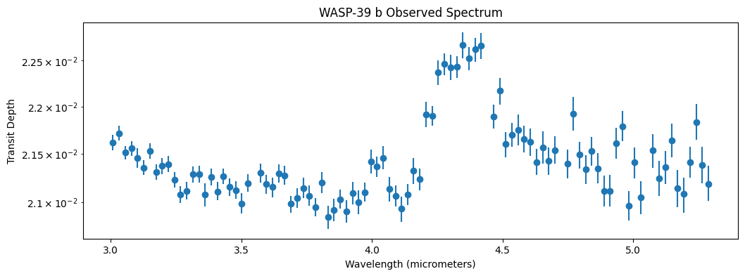
Before we start modeling a planet to match WASP-39 b, let’s get hold of WASP-39 b’s actual observed spectrum in data format, so we can plot it next to our modeled ones. If you did part 1 of this tutorial, you already downloaded the data prepared by the scientists who wrote the CO2 discovery paper.
Let’s practice download the data from Zenodo which is a popular place to host reduced data. Download the .zip, and then look for ZENODO/TRANSMISSION_SPECTRA_DATA/EUREKA_REDUCTION.txt.
[3]:
eureka_reduction_path = '/data2/observations/WASP-39b/ZENODO/TRANSMISSION_SPECTRA_DATA/EUREKA_REDUCTION.txt'
[4]:
# Import ascii
from astropy.io import ascii
# Confirm can read the file
observed_data = ascii.read(eureka_reduction_path)
[5]:
observed_data.colnames
[5]:
['wavelength',
'bin_width',
'tr_depth',
'tr_depth_errneg',
'tr_depth_errpos',
'ecl_depth',
'ecl_depth_errneg',
'ecl_depth_errpos']
Let’s plot the observed data and see what we are working with!
[6]:
plt=jpi.plt
plt.figure(figsize=(12,4))
plt.errorbar(observed_data['wavelength'], observed_data['tr_depth'],
[observed_data['tr_depth_errneg'], observed_data['tr_depth_errpos']],fmt='o')
plt.title('WASP-39 b Observed Spectrum')
plt.yscale('log')
plt.ylabel('Transit Depth')
plt.xlabel('Wavelength (micrometers)')
plt.show()
Spectra Ingredients
Now what? Let’s slowly build up a model that can match this data. What do we need?
PICASO Basics
List of what you will need before getting started
Planet properties
planet radius
planet mass
planet’s equilibrium temperature
Stellar properties
stellar log gravity
stellar effective temperature
stellar metallicity
Opacities (how do molecules and atoms absorb light under different pressure/temperature conditions)
Basic Inputs
Cross Section Connection
All rapid radiative transfer codes rely on a database of pre-computed cross sections. Cross sections are computed by using line lists in combination with critical molecular pressure broadening parameters. Both can either be derived from theoretical first principles (e.g., UCL ExoMol’s line lists), measured in a lab, and/or some combination thereof (e.g., HITRAN/HITEMP line lists).
When cross sections are initially computed, a resolution (\(\lambda/\Delta \lambda\)) is assumed. Cross sections are computed on a line-by-line nature and therefore usually computed for R~1e6. For JWST we are often interested in large bands (e.g. 1-14 \(\mu\)m). Therefore we need creative ways to speed up these runs. You will usually find one of two methods: correlated-k tables and resampled cross sections. Garland et al. 2019 is a good resource on the differences between these two.
For this demonstration we will use the resampled cross section method. The major thing to note about using resampled cross sections is that you have to compute your model at ~100x higher resolution than your data, but then must bin it down to a comparable resolution as your data so you can compare them. You will note that the opacity file you downloaded is resampled at R=10,000. Therefore you will note that in this tutorial we will always bin the model down to R=100 before comparing with the data.
The overall idea is that we are just simply initializing PICASO to operate, create a “connection” to the models/spectral tools, in that wavelength (in microns) with the respective opacity range.
[7]:
opa = jdi.opannection(wave_range=[2.7,6])
Set Basic Planet and Stellar Inputs
Second step is to define the basic planet parameters. Depending on the kind of model you want to compute (transmission vs. emission vs. reflected light), there are different requirements for the minimum set of information you need to include.
For WASP-39 b, since we have planet mass, radius, and all the necessary stellar specifications, we will be thorough in our inputs and include all parameters.
We can create an object called w39 that represents the planet WASP-39 b. We then assign values to that object. We already know the temperature, radius, metallicity, and surface gravity of the host star, so we can assign those values to the parent star under w39.star. We also know the mass and radius of the planet, so we can assign those values to the planet under w39.gravity (named thus because mass and radius will be used to compute the planet’s surface gravity). As we move through the tutorial and make climate models etc., we will be doing these calculations on the object w39.
[8]:
# Create that object or "case"
w39 = jdi.inputs()
# Describe the star
w39.star(opa, temp=5400 , database='phoenix',
metal=0.01, logg=4.45, radius=0.9, radius_unit=jdi.u.R_sun )
# Describe the planet
w39.gravity(mass=0.28, mass_unit=jdi.u.M_jup,
radius=1.27, radius_unit=jdi.u.R_jup)
[9]:
# To get information about a function, you can use '?'
help(w39.star)
Help on method star in module picaso.justdoit:
star(
opannection,
temp=None,
metal=None,
logg=None,
radius=None,
radius_unit=None,
semi_major=None,
semi_major_unit=None,
database='ck04models',
filename=None,
w_unit=None,
f_unit=None
) method of picaso.justdoit.inputs instance
Get the stellar spectrum using stsynphot and interpolate onto a much finer grid than the
planet grid.
Parameters
----------
opannection : class picaso.RetrieveOpacities
This is the opacity class and it's needed to get the correct wave info and raman scattering cross sections
temp : float
(Optional) Teff of the stellar model if using the stellar database feature.
Not needed for filename option.
metal : float
(Optional) Metallicity of the stellar model if using the stellar database feature.
Not needed for filename option.
logg : float
(Optional) Logg cgs of the stellar model if using the stellar database feature.
Not needed for filename option.
radius : float
(Optional) Radius of the star. Only needed as input if you want relative flux units (Fp/Fs)
radius_unit : astropy.unit
(Optional) Any astropy unit (e.g. `radius_unit=astropy.unit.Unit("R_sun")`)
semi_major : float
(Optional) Semi major axis of the planet. Only needed to compute fp/fs for albedo calculations.
semi_major_unit : astropy.unit
(Optional) Any astropy unit (e.g. `radius_unit=astropy.unit.Unit("au")`)
database : str
(Optional)The database to pull stellar spectrum from. See documentation for pysynphot.
Most popular are 'ck04models', phoenix' and
filename : str
(Optional) Upload your own stellar spectrum. File format = two column white space (wave, flux).
Must specify w_unit and f_unit
w_unit : str
(Optional) Astropy Unit
f_unit : str
(Optional) Astrpy Unit
[10]:
# want to see the spectrum you input? it lives here
w39.inputs['star']
[10]:
{'database': 'phoenix',
'temp': 5400,
'metal': 0.01,
'logg': 4.45,
'radius': np.float64(62613000000.0),
'radius_unit': 'cm',
'flux': array([7.69661116e+11, 7.67184922e+11, 7.64708505e+11, ...,
1.65050282e+13, 1.64692540e+13, 1.64120864e+13], shape=(7985,)),
'flux_unit': 'ergs cm^{-2} s^{-1} cm^{-1}',
'relative_flux': array([1., 1., 1., ..., 1., 1., 1.], shape=(7985,)),
'relative_flux_unit': '(Rs/Sa)^2 * ergs cm^{-2} s^{-1} cm^{-1}',
'wno': array([1666.8307186 , 1666.99741 , 1667.16411808, ..., 3702.9287111 ,
3703.29902248, 3703.6693709 ], shape=(7985,)),
'semi_major': nan,
'semi_major_unit': 'Semi Major axis not supplied',
'filename': None,
'w_unit': None,
'f_unit': None}
Set Climate and Chemistry
We now need to think about how we can model the climate and chemistry of this system. For the sake of this tutorial we will start really simple, then move forward to something more complex.
For climate, we will explore these levels in this tutorial
Isothermal (now)
Radiative-convective (next section)
For chemistry, we will explore these levels in this tutorial
Chemical Equilibrium
Pressure
If we imagine our “nlevels” as equally spaced altitude bands on the planet, then we will assign pressures to decrease logarithmically as altitude increases.
Gas is compressible and tends to behave in that way in planetary atmospheres (including on Earth).
[11]:
nlevels = 50
# Logspace goes from base^(start) to base^(end)
# so here we are going from 10^-6 to 10^2, which is
# 1 microbar to 100 bars of pressure.
# This is an arbitrarily chosen range, but this is the most common.
pressure = np.logspace(-6,2,nlevels)
[12]:
print(pressure)
[1.00000000e-06 1.45634848e-06 2.12095089e-06 3.08884360e-06
4.49843267e-06 6.55128557e-06 9.54095476e-06 1.38949549e-05
2.02358965e-05 2.94705170e-05 4.29193426e-05 6.25055193e-05
9.10298178e-05 1.32571137e-04 1.93069773e-04 2.81176870e-04
4.09491506e-04 5.96362332e-04 8.68511374e-04 1.26485522e-03
1.84206997e-03 2.68269580e-03 3.90693994e-03 5.68986603e-03
8.28642773e-03 1.20679264e-02 1.75751062e-02 2.55954792e-02
3.72759372e-02 5.42867544e-02 7.90604321e-02 1.15139540e-01
1.67683294e-01 2.44205309e-01 3.55648031e-01 5.17947468e-01
7.54312006e-01 1.09854114e+00 1.59985872e+00 2.32995181e+00
3.39322177e+00 4.94171336e+00 7.19685673e+00 1.04811313e+01
1.52641797e+01 2.22299648e+01 3.23745754e+01 4.71486636e+01
6.86648845e+01 1.00000000e+02]
Isothermal Temperature
Next we need to decide how the temperature of the atmosphere varies with pressure. On Earth, temperature generally drops as you travel further from the Earth’s surface, i.e. higher in altitude and lower in pressure. But that is not always the case. For simplicity, we’ll start by assuming the temperature of WASP-39 b’s atmosphere is constant with pressure, which is called “isothermal.” As our models get more sophisticated, we’ll be able to refer back to this simple case.
[13]:
# We can see from exo.MAST that the equilibrium temp
# of WASP 39 b is 1120 kelvin, so let's use a scale
# of temperatures based on that.
equilibrium_temperature = 1120.55
isothermal_temperature = np.zeros(nlevels) + equilibrium_temperature
[14]:
print(isothermal_temperature)
[1120.55 1120.55 1120.55 1120.55 1120.55 1120.55 1120.55 1120.55 1120.55
1120.55 1120.55 1120.55 1120.55 1120.55 1120.55 1120.55 1120.55 1120.55
1120.55 1120.55 1120.55 1120.55 1120.55 1120.55 1120.55 1120.55 1120.55
1120.55 1120.55 1120.55 1120.55 1120.55 1120.55 1120.55 1120.55 1120.55
1120.55 1120.55 1120.55 1120.55 1120.55 1120.55 1120.55 1120.55 1120.55
1120.55 1120.55 1120.55 1120.55 1120.55]
Setting the Atmosphere in PICASO
So far we have described the parent star and the planet. Now let’s define the planet’s atmosphere. Note, this is a common workflow, where you start by creating an object (w39) and then slowly add parameters (information) as you go.
[15]:
w39.atmosphere(df = jdi.pd.DataFrame({
'pressure':pressure,
'temperature':isothermal_temperature}))
[16]:
# want to see the input added to the class
w39.inputs['atmosphere']['profile']
[16]:
| pressure | temperature | |
|---|---|---|
| 0 | 0.000001 | 1120.55 |
| 1 | 0.000001 | 1120.55 |
| 2 | 0.000002 | 1120.55 |
| 3 | 0.000003 | 1120.55 |
| 4 | 0.000004 | 1120.55 |
| 5 | 0.000007 | 1120.55 |
| 6 | 0.000010 | 1120.55 |
| 7 | 0.000014 | 1120.55 |
| 8 | 0.000020 | 1120.55 |
| 9 | 0.000029 | 1120.55 |
| 10 | 0.000043 | 1120.55 |
| 11 | 0.000063 | 1120.55 |
| 12 | 0.000091 | 1120.55 |
| 13 | 0.000133 | 1120.55 |
| 14 | 0.000193 | 1120.55 |
| 15 | 0.000281 | 1120.55 |
| 16 | 0.000409 | 1120.55 |
| 17 | 0.000596 | 1120.55 |
| 18 | 0.000869 | 1120.55 |
| 19 | 0.001265 | 1120.55 |
| 20 | 0.001842 | 1120.55 |
| 21 | 0.002683 | 1120.55 |
| 22 | 0.003907 | 1120.55 |
| 23 | 0.005690 | 1120.55 |
| 24 | 0.008286 | 1120.55 |
| 25 | 0.012068 | 1120.55 |
| 26 | 0.017575 | 1120.55 |
| 27 | 0.025595 | 1120.55 |
| 28 | 0.037276 | 1120.55 |
| 29 | 0.054287 | 1120.55 |
| 30 | 0.079060 | 1120.55 |
| 31 | 0.115140 | 1120.55 |
| 32 | 0.167683 | 1120.55 |
| 33 | 0.244205 | 1120.55 |
| 34 | 0.355648 | 1120.55 |
| 35 | 0.517947 | 1120.55 |
| 36 | 0.754312 | 1120.55 |
| 37 | 1.098541 | 1120.55 |
| 38 | 1.599859 | 1120.55 |
| 39 | 2.329952 | 1120.55 |
| 40 | 3.393222 | 1120.55 |
| 41 | 4.941713 | 1120.55 |
| 42 | 7.196857 | 1120.55 |
| 43 | 10.481131 | 1120.55 |
| 44 | 15.264180 | 1120.55 |
| 45 | 22.229965 | 1120.55 |
| 46 | 32.374575 | 1120.55 |
| 47 | 47.148664 | 1120.55 |
| 48 | 68.664885 | 1120.55 |
| 49 | 100.000000 | 1120.55 |
Chemistry
Now we need to add the chemistry! PICASO has a prebuilt chemistry table that was computed by Channon Visscher. You can use it by adding it to your input case. Two more chemistry parameters are now going to be introduced:
M/H: Atmospheric metallicity
C/O ratio: Elemental carbon to oxygen ratio
Metallicity

Looking at a mass-metallicity plot (compiled in Wakeford & Dalba 2020) might offer a good starting point to decide what the M/H of your planet might be. Here we can see WASP-39 b HST observations led to the inference of ~100xM/H. One tactic might be to start from that estimate. Another might be to use the Solar System extrapolated value (gray dashed line) as a first pass. Let’s start with the latter as a first guess.
[17]:
log_mh = 1.0 # log relative to solar
# so a value of 1 here represents 10^1 = 10x solar
C/O Ratio
The elemental ratio of carbon to oxygen controls the dominant carbon-bearing species. For instance, take a look at Figure 1 from the paper C/O RATIO AS A DIMENSION FOR CHARACTERIZING EXOPLANETARY ATMOSPHERES.
At low C/O, we see CO\(_2\) and CO as the dominant form of carbon, and at high C/O we see CH\(_4\) and CO as the dominant form of carbon.
C/O is given in PICASO in units relative to solar C/O, which is worth noting because you’re not giving it the actual ratio of carbon to oxygen, but rather the ratio relative to the Solar C/O. Solar C/O is ~0.5 (Asplund et al. 2021), and let’s set our value to be the same as Solar (i.e. 1 relative to Solar).
[18]:
c_o = 0.55 # absolute solar
Now we can ask PICASO to make us a mixture of molecules consistent with the relative M/H metallicity and relative C/O ratio we set up, and we can take a look at what it creates. We can look at the “atmosphere profile” which shows us the abundances of various molecules at different levels of our atmosphere (levels being places where temperature and pressure differ in the manner we defined above).
This can help us find out which molecules we should really focus on during our analysis, and others that may be harder or redundant to look for based off of our C/O ratio and metallicity.
[19]:
w39.chemeq_visscher_2121(c_o, log_mh)
Running this function sets a dataframe in your inputs dictionary, which you can access now with w39.inputs['atmosphere']['profile']. You can see that PICASO has given us loads of different molecules to work with, but many have miniscule abundances (note some e-38 values in there).
[20]:
w39.inputs['atmosphere']['profile'].head()
[20]:
| pressure | temperature | e- | H2 | H | H+ | H- | H2- | H2+ | H3+ | ... | LiF | C | O | Mg | Mg+ | Si | Fe+ | Ti | Ti+ | C+ | |
|---|---|---|---|---|---|---|---|---|---|---|---|---|---|---|---|---|---|---|---|---|---|
| 0 | 0.000001 | 1120.55 | 9.381468e-10 | 0.824024 | 0.000037 | 1.073912e-49 | 1.516359e-18 | 8.670002e-28 | 2.270187e-50 | 1.557381e-41 | ... | 2.990005e-10 | 6.624051e-27 | 3.156146e-14 | 2.489242e-08 | 6.068341e-26 | 4.513898e-19 | 3.111704e-25 | 2.296944e-21 | 2.556457e-35 | 1.000000e-50 |
| 1 | 0.000001 | 1120.55 | 7.700674e-10 | 0.824025 | 0.000030 | 9.895630e-50 | 1.502156e-18 | 1.036543e-27 | 2.180260e-50 | 1.572103e-41 | ... | 3.224939e-10 | 6.624220e-27 | 2.166915e-14 | 1.709082e-08 | 3.485000e-26 | 3.099261e-19 | 1.786983e-25 | 1.577076e-21 | 1.468166e-35 | 1.000000e-50 |
| 2 | 0.000002 | 1120.55 | 6.321013e-10 | 0.824026 | 0.000025 | 9.118392e-50 | 1.488086e-18 | 1.239241e-27 | 2.093896e-50 | 1.586964e-41 | ... | 3.478332e-10 | 6.624389e-27 | 1.487739e-14 | 1.173435e-08 | 2.001408e-26 | 2.127965e-19 | 1.026225e-25 | 1.082816e-21 | 8.431631e-36 | 1.000000e-50 |
| 3 | 0.000003 | 1120.55 | 5.188285e-10 | 0.824027 | 0.000021 | 8.402567e-50 | 1.474066e-18 | 1.481483e-27 | 2.011036e-50 | 1.602056e-41 | ... | 3.756413e-10 | 6.624533e-27 | 1.021455e-14 | 8.056750e-09 | 1.149477e-26 | 1.461080e-19 | 5.893845e-26 | 7.434653e-22 | 4.842606e-36 | 1.000000e-50 |
| 4 | 0.000004 | 1120.55 | 4.256149e-10 | 0.824028 | 0.000017 | 7.746897e-50 | 1.459220e-18 | 1.769753e-27 | 1.932395e-50 | 1.618358e-41 | ... | 4.117899e-10 | 6.624374e-27 | 7.014576e-15 | 5.532500e-09 | 6.607562e-27 | 1.003279e-19 | 3.388062e-26 | 5.105194e-22 | 2.783626e-36 | 1.000000e-50 |
5 rows × 52 columns
Reference Pressure
Lastly, we need to decide on a “reference pressure.” If our planet was terrestrial, this would be the pressure at the surface, and therefore also the pressure corresponding to the radius of the planet. For gas giants like WASP-39 b, this is a bit more complicated – there is no “surface,” so we need to pick a pressure that corresponds to our planet’s “radius” or surface, so that PICASO can calculate gravity as a function of altitude from that level.
We are selecting a pressure that we are essentially calling the bottom.
As we’ve discussed, a planet’s radius changes depending on the wavelength at which you observe it – it’s that change that we are measuring with our spectra. But when we input the planet radius above, we picked a single number – 1.27 r_jup. That number is an average calculated over a band of wavelengths. And so when we pick a reference pressure, we estimate roughly what level of the planet’s atmosphere that averaged radius corresponds to (where, from the high pressure deep inside, to the
low pressure at the exterior, does the chosen radius fall?).
PICASO suggests a reference pressure of 10 bar for gas giants, so we will start with that:
[21]:
w39.approx(p_reference=10)
Want to check your inputs so far?
If you want you can consult w39.inputs to check or reset inputs. Let’s see how our WASP-39 b object is holding up!
[22]:
w39.inputs.keys()
[22]:
dict_keys(['version', 'calculation', 'phase', 'planet', 'climate', 'star', 'atmosphere', 'clouds', 'approx', 'disco', 'opacities', 'test_mode'])
An atmosphere profile table shows the elemental abundances at each pressure level in our model atmosphere.
[23]:
w39.inputs['atmosphere']['profile'].head()
[23]:
| pressure | temperature | e- | H2 | H | H+ | H- | H2- | H2+ | H3+ | ... | LiF | C | O | Mg | Mg+ | Si | Fe+ | Ti | Ti+ | C+ | |
|---|---|---|---|---|---|---|---|---|---|---|---|---|---|---|---|---|---|---|---|---|---|
| 0 | 0.000001 | 1120.55 | 9.381468e-10 | 0.824024 | 0.000037 | 1.073912e-49 | 1.516359e-18 | 8.670002e-28 | 2.270187e-50 | 1.557381e-41 | ... | 2.990005e-10 | 6.624051e-27 | 3.156146e-14 | 2.489242e-08 | 6.068341e-26 | 4.513898e-19 | 3.111704e-25 | 2.296944e-21 | 2.556457e-35 | 1.000000e-50 |
| 1 | 0.000001 | 1120.55 | 7.700674e-10 | 0.824025 | 0.000030 | 9.895630e-50 | 1.502156e-18 | 1.036543e-27 | 2.180260e-50 | 1.572103e-41 | ... | 3.224939e-10 | 6.624220e-27 | 2.166915e-14 | 1.709082e-08 | 3.485000e-26 | 3.099261e-19 | 1.786983e-25 | 1.577076e-21 | 1.468166e-35 | 1.000000e-50 |
| 2 | 0.000002 | 1120.55 | 6.321013e-10 | 0.824026 | 0.000025 | 9.118392e-50 | 1.488086e-18 | 1.239241e-27 | 2.093896e-50 | 1.586964e-41 | ... | 3.478332e-10 | 6.624389e-27 | 1.487739e-14 | 1.173435e-08 | 2.001408e-26 | 2.127965e-19 | 1.026225e-25 | 1.082816e-21 | 8.431631e-36 | 1.000000e-50 |
| 3 | 0.000003 | 1120.55 | 5.188285e-10 | 0.824027 | 0.000021 | 8.402567e-50 | 1.474066e-18 | 1.481483e-27 | 2.011036e-50 | 1.602056e-41 | ... | 3.756413e-10 | 6.624533e-27 | 1.021455e-14 | 8.056750e-09 | 1.149477e-26 | 1.461080e-19 | 5.893845e-26 | 7.434653e-22 | 4.842606e-36 | 1.000000e-50 |
| 4 | 0.000004 | 1120.55 | 4.256149e-10 | 0.824028 | 0.000017 | 7.746897e-50 | 1.459220e-18 | 1.769753e-27 | 1.932395e-50 | 1.618358e-41 | ... | 4.117899e-10 | 6.624374e-27 | 7.014576e-15 | 5.532500e-09 | 6.607562e-27 | 1.003279e-19 | 3.388062e-26 | 5.105194e-22 | 2.783626e-36 | 1.000000e-50 |
5 rows × 52 columns
We can look at the abundances for a single molecule, say CO\(_2\).
[24]:
# Grab CO2 array, for instance
w39.inputs['atmosphere']['profile']['CO2'].values
[24]:
array([1.93501557e-05, 1.93498225e-05, 1.93494894e-05, 1.93492469e-05,
1.93500715e-05, 1.93508962e-05, 1.93517208e-05, 1.93522092e-05,
1.93526496e-05, 1.93530899e-05, 1.93534105e-05, 1.93537252e-05,
1.93540400e-05, 1.93544489e-05, 1.93548893e-05, 1.93553296e-05,
1.93554052e-05, 1.93554052e-05, 1.93554052e-05, 1.93554647e-05,
1.93555599e-05, 1.93556552e-05, 1.93558437e-05, 1.93560716e-05,
1.93562995e-05, 1.93578349e-05, 1.93606782e-05, 1.93635219e-05,
1.93814927e-05, 1.94105249e-05, 1.94396006e-05, 1.95398451e-05,
1.97603408e-05, 1.99833247e-05, 2.03361887e-05, 2.08526416e-05,
2.13822102e-05, 2.12394525e-05, 1.91792514e-05, 1.73188873e-05,
1.39808628e-05, 8.97417164e-06, 5.76042822e-06, 3.58937246e-06,
1.81679443e-06, 9.19587487e-07, 4.59750946e-07, 2.19011047e-07,
1.04330049e-07, 4.96995892e-08])
We can check our inputs for the planet and the host star.
[25]:
w39.inputs['planet'], w39.inputs['star'] # All your inputs have been archived!
[25]:
({'gravity': np.float64(430.29483869562654),
'gravity_unit': 'cm/(s**2)',
'radius': np.float64(9079484000.0),
'radius_unit': 'cm',
'mass': np.float64(5.3147488725409414e+29),
'mass_unit': 'g'},
{'database': 'phoenix',
'temp': 5400,
'metal': 0.01,
'logg': 4.45,
'radius': np.float64(62613000000.0),
'radius_unit': 'cm',
'flux': array([7.69661116e+11, 7.67184922e+11, 7.64708505e+11, ...,
1.65050282e+13, 1.64692540e+13, 1.64120864e+13], shape=(7985,)),
'flux_unit': 'ergs cm^{-2} s^{-1} cm^{-1}',
'relative_flux': array([1., 1., 1., ..., 1., 1., 1.], shape=(7985,)),
'relative_flux_unit': '(Rs/Sa)^2 * ergs cm^{-2} s^{-1} cm^{-1}',
'wno': array([1666.8307186 , 1666.99741 , 1667.16411808, ..., 3702.9287111 ,
3703.29902248, 3703.6693709 ], shape=(7985,)),
'semi_major': nan,
'semi_major_unit': 'Semi Major axis not supplied',
'filename': None,
'w_unit': None,
'f_unit': None})
Creating a Transmission Spectrum
Now that we have set up PICASO with everything it needs, and we understand the components needed to model an exoplanet, let’s ask PICASO to output a transmission spectrum for our WASP-39 b.
First Run PICASO
We can use the .spectrum function to do so.
We need to give the function a connection to the opacity database we used earlier to look up the absorption spectrum for water, as well as an instruction to create a “transmission” spectrum (as opposed to, for example, a reflected light spectrum of star light bouncing off the planet when it’s almost behind its star).
[26]:
model_iso = w39.spectrum(opa,
# Other options are "thermal" or "reflected"
# or a combination of two e.g. "transmission+thermal"
calculation='transmission',
full_output=True)
Our Spectra
Let’s set up a function to display the spectrum in our first output dictionary (first one is called model_iso). Moving forward we will create more models and we want a way to easily display them.
[27]:
def show_spectra(output, x_range_min=3.0, x_range_max=5.5):
# Step 1) Regrid model to be on the same x axis as the data
wnos, transit_depth = jdi.mean_regrid(output['wavenumber'],
output['transit_depth'],
newx=sorted(1e4/observed_data['wavelength']))
# Step 2) Use PICASO function to create a plot with the models
fig = jpi.spectrum(wnos, transit_depth,
plot_width=800,y_axis_label='Absolute (Rp/Rs)^2',
x_range=(x_range_min,x_range_max))
# Step 3) Use PICASO function to add the data so we can compare
jpi.plot_multierror(observed_data['wavelength'], observed_data['tr_depth'], fig,
dy_low=observed_data['tr_depth_errneg'], dy_up=observed_data['tr_depth_errpos'],
dx_low=[0],dx_up=[0], point_kwargs={'color':'black'})
jpi.show(fig)
[28]:
# Display our first spectrum!
show_spectra(model_iso)
Sweet! We have a spectrum that looks the right-ish shape, even though it isn’t quite in the right place. Let’s take a minute to work that out.
Transit Depth Offsets
Remember how we guessed what the reference pressure was? Well, it looks like we are a little off. That is okay! When fitting for transit spectra, we introduce a factor to account for this. In the retrieval tutorial, you will fit for a factor of the radius. For now, let’s “mean subtract” our data so that the model and data lie on top of one another.
[29]:
# Let's mean subtract these
def show_spectra(output, x_range_min=3.0, x_range_max=5.5):
# Step 1) Regrid model to be on the same x axis as the data
wnos, transit_depth = jdi.mean_regrid(output['wavenumber'],
output['transit_depth'],
newx=sorted(1e4/observed_data['wavelength']))
# Step 2) Use PICASO function to create a plot with the models
fig = jpi.spectrum(wnos, transit_depth-np.mean(transit_depth),
plot_width=800, y_axis_label='Relative (Rp/Rs)^2',
x_range=(x_range_min,x_range_max))
# Step 3) Use PICASO function to add the data so we can compare
jpi.plot_multierror(observed_data['wavelength'],
observed_data['tr_depth'] - np.mean(observed_data['tr_depth']),
fig,
dy_low=observed_data['tr_depth_errneg'], dy_up=observed_data['tr_depth_errpos'],
dx_low=[0],dx_up=[0], point_kwargs={'color':'black'})
jpi.show(fig)
[30]:
show_spectra(model_iso)
Model Investigation
Before trying to improve the complexity of your model, let’s make sure you know how to analyze the inputs.
Identifying molecular features with optical depth contribution plot
taus_per_layer - Each dictionary entry is a nlayer x nwave that represents the per layer optical depth for that molecule.
cumsum_taus - Each dictionary entry is a nlevel x nwave that represents the cumulative summed opacity for that molecule.
tau_p_surface - Each dictionary entry is a nwave array that represents the pressure level where the cumulative opacity reaches the value specified by the user through at_tau.
Let’s create a molecule contribution plot. At any given wavelength, this will show us at which pressure layer (tau_p_surface) each molecule experiences an optical depth of \(\tau\). Below, we will set \(\tau = 1\). This is useful because whenever we see a spectral feature, that light is originating from a depth in the atmosphere corresponding to the \(\tau=1\) surface for that molecule.
[31]:
molecule_contribution = jdi.get_contribution(w39, opa, at_tau=1)
[32]:
jpi.show(jpi.molecule_contribution(molecule_contribution,
opa, plot_width=700, x_axis_type='log'))
Identifying molecular features with “leave-one-out” method
Another option for investigating model output is to remove the contribution of one gas from the model to see if it affects our spectrum. CO\(_2\) was a fairly obvious feature for the 4.3\(\mu\)m. But what about H\(_2\)O and CO from 4.4-6\(\mu\)m. In this region there is no distinct “feature” in the spectrum. How sure are we that H\(_2\)O and CO are really there? We can use the “leave-one-out” method to see how individual molecules are shaping each part of our spectrum.
We can use PICASO’s exclude_mol key to exclude the optical contribution from one molecule at a time. In the code below lets do this for CO2, H2O, and CO. We will loop through one by one and create a spectra without each of these. The result will show you where their contribution to the spectra is most important.
[33]:
w,f,l =[],[],[]
df_og = jdi.copy.deepcopy(w39.inputs['atmosphere']['profile'])
for iex in ['CO2','H2O','CO',None]:
w39.atmosphere(df=df_og,exclude_mol=iex, sep=r'\s+')
df= w39.spectrum(opa, full_output=True,calculation='transmission') #note the new last key
wno, rprs2 = df['wavenumber'] , df['transit_depth']
wno, rprs2 = jdi.mean_regrid(wno, rprs2, R=150)
w +=[wno]
f +=[rprs2]
if iex==None:
leg='all'
else:
leg = f'No {iex}'
l+=[leg]
jpi.show(jpi.spectrum(w,f,legend=l))
We can see clearly that when H\(_2\)O or CO\(_2\) is not present, a completely different spectrum is created that veers far from our model. Therefore we can feel confident that H\(_2\)O or CO\(_2\) are truly present. When we try leaving out CO, however, the spectrum changes more modestly; it appears that including CO improves the spectrum somewhat, but we are less certain about its presence.
Increasing Model Complexity to Improve Fit: Chemistry, Climate, Clouds
In the next sections we will try to improve our model fit. However, before we continue we need a way to quantify our “goodness of fit.”
Define Goodness of Fit
Let’s implement a simple measurement of error called a “chi-squared test.” This is a commonly used method to measure how well you are fitting data with a model, and sums up the distance between your model’s output and the observed data at each data point.
The standard chi-squared test formula is \(\chi^2 = \sum \frac{(O_i - E_i)^2}{(\sigma_i)^2}\) where \(O\) is the observed data, \(E\) is the expected value (i.e. our model), and \(\sigma\) is error.
In this notebook, we’ll compute chi-squared per data point, which means we are normalizing the standard chi-square by dividing by number of data points. The chi-squared per data point formula is \(\frac{\chi^2}{N}\) where \(N\) is the number of data points.
Note, another common way to report chi-squared is the reduced chi-squared which considers the degrees of freedom \((\nu)\), where \(\nu\) is the number of data points (\(N\)) minus the number of fitted parameters.
Regardless of the version of chi-squared you use, if the result is close to 1, that is considered a good fit.
[34]:
def chisqr(model):
# Step 1) Regrid model to be on the same x axis as the data
wnos, model_binned = jdi.mean_regrid(model['wavenumber'],
model['transit_depth'],
newx=sorted(1e4/observed_data['wavelength']))
# Step 2) Flip model so that it is increasing with wavelength, not wavenumber
model_binned = model_binned[::-1]-np.mean(model_binned)
# Step 3) Compute chi sq with mean subtraction
observed = observed_data['tr_depth'] - np.mean(observed_data['tr_depth'])
error = (observed_data['tr_depth_errneg'] + observed_data['tr_depth_errpos'])/2
return np.sum(((observed-model_binned)/error)**2 ) / len(model_binned)
[35]:
print('Simple First Guess', chisqr(model_iso))
Simple First Guess 14.487825120956886
Not great! Let’s make it better.
Revisiting Chemistry Assumption
Earlier, we assumed M/H and C/O values. Let’s loop through a few M/H and C/O values to see if any of these seem to improve our model fit. Why? These values are faster to assess than climate or clouds, and they’re easier to loop through while you’re building intuition. We want to find the best fit combination of variables such as C/O and M/H that will gives us the closest fit to the data.
[36]:
mh_grid_vals = [1, 10, 100]
co_grid_vals = [0.55, 1.3] #absolute c/o ratios
chemistry_grid = {}
for imh in mh_grid_vals:
for ico in co_grid_vals:
w39.chemeq_visscher_2121(ico, np.log10(imh))
chemistry_grid[f'M/H={imh},C/O={ico}'] = w39.spectrum(opa, calculation='transmission', full_output=True)
print(f'M/H={imh},C/O={ico}', chisqr(chemistry_grid[f'M/H={imh},C/O={ico}'] ))
M/H=1,C/O=0.55 12.030864097989959
M/H=1,C/O=1.3 45.09445251738913
M/H=10,C/O=0.55 14.487825120956886
M/H=10,C/O=1.3 30.01359267397018
M/H=100,C/O=0.55 3.5656165090244016
M/H=100,C/O=1.3 12.208643609034011
We see with a M/H of 100 and C/O of 1, we get the best fit where the chi-squared is ~4. Let’s plot all these and visually confirm.
[37]:
# Let's edit our function once again to allow for multiple model inputs
def show_spectra(output, x_range_min=3.0, x_range_max=5.5):
#Step 1) Regrid model to be on the same x axis as the data
wnos, transit_depth = zip(*[jdi.mean_regrid(output[x]['wavenumber'], output[x]['transit_depth'],
newx=sorted(1e4/observed_data['wavelength']))
for x in output])
transit_depth = [x-np.min(x) for x in transit_depth]
wnos = [x for x in wnos]
legends = [i for i in output]
# Step 2) Use picaso function to create a plot with the models
fig = jpi.spectrum(wnos, transit_depth, legend=legends,
plot_width=800,y_axis_label='Relative (Rp/Rs)^2',
x_range=(x_range_min,x_range_max))
# Step 3) Use picaso function to add the data so we can compare
jpi.plot_multierror(observed_data['wavelength'],
observed_data['tr_depth'] - np.min(observed_data['tr_depth']),
fig,
dy_low=observed_data['tr_depth_errneg'], dy_up=observed_data['tr_depth_errpos'],
dx_low=[0], dx_up=[0], point_kwargs={'color':'black'})
jpi.show(fig)
[38]:
show_spectra(chemistry_grid)
Check your understanding
Let’s investigate how our chemistry choices affect our model spectrum. Explore the figure above by clicking on the legend to remove different lines.
Try looking only at lines that keep C/O steady while varying M/H from 1 to 10 to 100. What impact does the change in M/H ratio have on the spectrum?
You’ll notice that as M/H increases, the CO\(_2\) bump near 4.4 \(\mu\)m initially grows and then shrinks. Why might this be?
Now look at lines that keep M/H steady while varying C/O from 1 to 2.5. What impact does this change in C/O ratio have on the spectrum?
You’ll notice that as C/O increases, the CO\(_2\) bump near 4.4 \(\mu\)m disappears while a new CH\(_4\) line appears near 3.35 \(\mu\)m. Why might this be?
Some more targeted questions to help with the above:
Figure out what the top 4 most abundant oxygen- and carbon-bearing species are by looking at your chemistry grid.
How does their abundance change when you vary the value of M/H?
How does their abundance change when we increase C/O from 1 to 2.5?
How does mean the atmosphere’s molecular weight change when you vary M/H?
Can you see that reflected in the spectrum?
Solution 1: Figure out what the top 4 most abundant oxygen- and carbon-bearing species are by looking at your chemistry grid.
Let’s write a simple function to find the most abundance O and C bearing species
[39]:
# Write a simple function to identify the top most abundant species
def find_top(grid, mh=1, co=0.55, n=4, method='average', more=False):
"""
Find the n most abundant oxygen- and carbon-bearing molecules for a given M/H and C/O ratio.
Parameters
----------
grid: dict
chemistry grid"
mh : int (optional)
M/H ratio relative to Solar
co : int (optional)
C/O ratio relative to Solar
n : int (optional)
number of molecules you want to identify
method : str (optional)
how you will calculate the abundance of a given species; options are 'sum', 'average', 'median'
more : boolean (optional)
if True, will print results of each step
Returns
-------
top_dict
dictionary of the most abundant C- and O-bearing molecules and their total abundances
"""
# What are all the available species? (elements start in fourth column)
cols = grid[f'M/H={mh},C/O={co}']['full_output']['layer']['mixingratios'].columns.tolist()[3::]
if more == True:
print("All available species:\n", cols, "\n")
# Grab only the carbon- and/or oxygen-bearing molecules
filtered_cols = [mol for mol in cols if ('C' in mol or 'O' in mol) and 'Cs' not in mol]
if more == True:
print("Carbon- and/or oxygen-bearing molecules:\n", filtered_cols, "\n")
# Choose a value to represent the abundance for each molecule
tot_abun = {}
for mol in filtered_cols:
if method == 'sum': # Sum the abundance across all pressure layers
tot_abun[mol] = np.sum(grid[f'M/H={mh},C/O={co}']['full_output']['layer']['mixingratios'][mol].values)
elif method == 'average': # Choose the average abundance value
tot_abun[mol] = np.average(grid[f'M/H={mh},C/O={co}']['full_output']['layer']['mixingratios'][mol].values)
elif method == 'median': # Choose the median abundance value
tot_abun[mol] = np.median(grid[f'M/H={mh},C/O={co}']['full_output']['layer']['mixingratios'][mol].values)
if more == True:
print("Total abundances:\n", tot_abun, "\n")
# What are the 4 highest abundances?
top = sorted(tot_abun, key=tot_abun.get, reverse=True)[:n]
top_dict = {k: tot_abun[k] for k in top}
if more == True:
print(f"Top {n} carbon- and/or oxygen-bearing molecules:\n", top)
return top_dict
# Uncomment to test
find_top(chemistry_grid, method='average', more=True)
All available species:
['H+', 'H-', 'H2-', 'H2+', 'H3+', 'He', 'H2O', 'CH4', 'CO', 'NH3', 'N2', 'PH3', 'H2S', 'TiO', 'VO', 'Fe', 'FeH', 'CrH', 'Na', 'K', 'Rb', 'atCs', 'CO2', 'HCN', 'C2H2', 'C2H4', 'C2H6', 'SiO', 'MgH', 'COS', 'Li', 'LiOH', 'LiH', 'LiCl', 'OH', 'C-gr', 'Li+', 'LiF', 'C', 'O', 'Mg', 'Mg+', 'Si', 'Fe+', 'Ti', 'Ti+', 'C+']
Carbon- and/or oxygen-bearing molecules:
['H2O', 'CH4', 'CO', 'TiO', 'VO', 'CrH', 'CO2', 'HCN', 'C2H2', 'C2H4', 'C2H6', 'SiO', 'COS', 'LiOH', 'LiCl', 'OH', 'C-gr', 'C', 'O', 'C+']
Total abundances:
{'H2O': np.float64(0.00045579747317718296), 'CH4': np.float64(0.00015736319593958136), 'CO': np.float64(0.00043475202411969973), 'TiO': np.float64(9.699957360028092e-16), 'VO': np.float64(3.076549577132749e-13), 'CrH': np.float64(1.4820765864739592e-13), 'CO2': np.float64(1.540725988531297e-07), 'HCN': np.float64(1.0509143111934562e-09), 'C2H2': np.float64(8.426156717253372e-13), 'C2H4': np.float64(2.952956863650337e-11), 'C2H6': np.float64(4.5072271775875076e-11), 'SiO': np.float64(4.1356142256885574e-08), 'COS': np.float64(6.565498492390416e-10), 'LiOH': np.float64(6.056412432295548e-10), 'LiCl': np.float64(2.585506493240405e-09), 'OH': np.float64(9.124145782227813e-12), 'C-gr': np.float64(9.999999999999953e-51), 'C': np.float64(4.55829950814816e-27), 'O': np.float64(1.777829599387293e-16), 'C+': np.float64(9.999999999999953e-51)}
Top 4 carbon- and/or oxygen-bearing molecules:
['H2O', 'CO', 'CH4', 'CO2']
[39]:
{'H2O': np.float64(0.00045579747317718296),
'CO': np.float64(0.00043475202411969973),
'CH4': np.float64(0.00015736319593958136),
'CO2': np.float64(1.540725988531297e-07)}
Solution 2: How do abundances change when varying M/H?
[40]:
# Visualize how the abundance of each molecule changes as M/H increases
# Initialize an empty dictionary to store abundances
abundances = {}
# Loop through the M/H grid values
for i, mh in enumerate(mh_grid_vals):
# Calculate total abundance of top 4 molecules for a given M/H value
top_dict = find_top(chemistry_grid, mh=mh, co=0.55, n=5, method='sum')
print(f'M/H={mh}, C/O=1:', top_dict)
# Add molecule abundances dynamically and insert at the correct position
for molecule, abundance in top_dict.items():
if molecule not in abundances:
abundances[molecule] = [None] * len(mh_grid_vals) # Initialize the list with None
abundances[molecule][i] = abundance # Insert the abundance at the correct index
# Plot abundance vs. M/H for top 4 molecules
plt.figure(figsize=(8, 4), dpi=100)
for molecule in abundances:
plt.plot(mh_grid_vals, abundances[molecule], marker='o', label=molecule)
plt.yscale('log')
plt.xscale('log')
plt.xlabel('M/H (xSolar)')
plt.ylabel('Total Abundance')
plt.legend()
plt.show()
M/H=1, C/O=1: {'H2O': np.float64(0.022334076185681964), 'CO': np.float64(0.021302849181865285), 'CH4': np.float64(0.007710796601039487), 'CO2': np.float64(7.549557343803356e-06), 'SiO': np.float64(2.026450970587393e-06)}
M/H=10, C/O=1: {'CO': np.float64(0.22959714259137545), 'H2O': np.float64(0.2027714691241707), 'CH4': np.float64(0.05841534879922737), 'CO2': np.float64(0.0008059161818930456), 'COS': np.float64(3.4154822877455008e-06)}
M/H=100, C/O=1: {'CO': np.float64(2.28590562452462), 'H2O': np.float64(1.6575613034599495), 'CH4': np.float64(0.36754402032565114), 'CO2': np.float64(0.07983960633341423), 'COS': np.float64(0.00032474616443891826)}
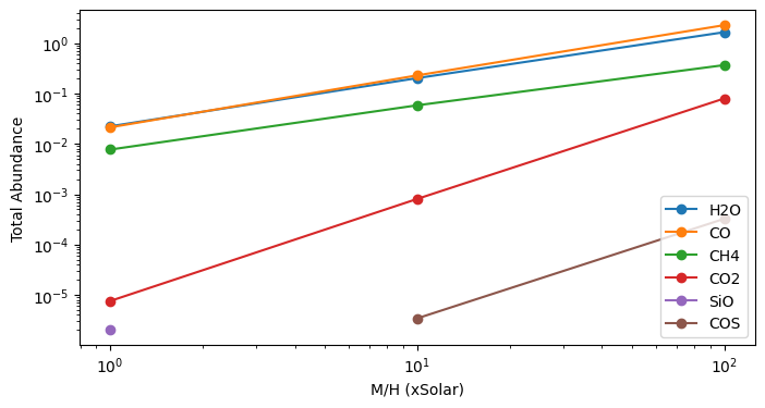
We see that most species increase in abundance as metallicity increases, and they do so at different rates.
Solution 3: How do abundances change when varying C/O?
[41]:
# Visualize how the abundance of each molecule changes as C/O increases
# Initialize an empty dictionary to store abundances
abundances = {}
# Loop through the C/O grid values
for i, co in enumerate(co_grid_vals):
# Calculate total abundance of top 4 molecules for a given C/O value
top_dict = find_top(chemistry_grid, mh=1, co=co, method='sum')
print(f'M/H=1, C/O={co}:', top_dict)
# Add molecule abundances dynamically and insert at the correct position
for molecule, abundance in top_dict.items():
if molecule not in abundances:
abundances[molecule] = [None] * len(co_grid_vals) # Initialize the list with None
abundances[molecule][i] = abundance # Insert the abundance at the correct index
# Plot abundance vs. C/O for top 4 molecules
plt.figure(figsize=(8, 4), dpi=100)
for molecule in abundances:
plt.plot(co_grid_vals, abundances[molecule], marker='o', label=molecule)
plt.xlabel("C/O (xSolar)")
plt.ylabel("Total Abundance")
plt.legend()
plt.show()
M/H=1, C/O=0.55: {'H2O': np.float64(0.022334076185681964), 'CO': np.float64(0.021302849181865285), 'CH4': np.float64(0.007710796601039487), 'CO2': np.float64(7.549557343803356e-06)}
M/H=1, C/O=1.3: {'CO': np.float64(0.024554340173318537), 'CH4': np.float64(0.015295373743119258), 'H2O': np.float64(0.007815071922496405), 'C-gr': np.float64(0.0031332660510965146)}
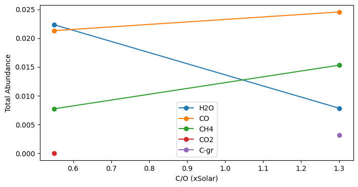
We see that as the ratio of carbon to oxygen increases, the abundance of carbon-bearing species (CH\(_4\) and CO) grows while the abundance of H\(_2\)O declines.
Solution 4: How does mean molecular weight vary with M/H?
[42]:
# Visualize how mean molecular weight changes with M/H
# Get the average mean molecular weight of the atmosphere at each M/H value
mmws = []
for mh in mh_grid_vals:
mmws.append(np.mean(chemistry_grid[f'M/H={mh},C/O=0.55']['full_output']['layer']['mmw']))
# Plot how the mean molecular weight of each molecules changes with M/H
plt.figure(figsize=(8, 4), dpi=100)
plt.plot(mh_grid_vals, mmws, marker='o')
#plt.xscale('log')
plt.xlabel('M/H (xSolar)')
plt.ylabel('Mean $\\mu$')
plt.show()
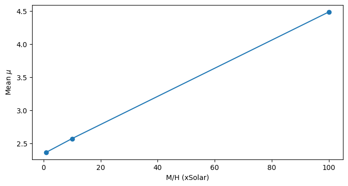
We see that mean molecular weight increases linearly as M/H increases.
Step 5: Can you see this reflected in the spectrum? What impact does the change in M/H ratio have on the spectrum?
Click to expand solution
Why a feature might grow: The strength of a spectral feature is impacted by a molecule’s abundance. When we increase atmospheric metallicity, we are increasing the raw abundance of all elements heavier than hydrogen. Complicated chemical processes ensue, resulting in a new distribution of molecules constructed from those raw elements. Some molecules (e.g., CO\(_2\)) are more sensitive to changes in metallicity than others (e.g., H\(_2\)O), so although the abundance of all molecules will increase as metallicity increases, they will do so at different rates. Why a feature might shrink: The strength of all spectral features is tied to the scale height of the atmosphere. Scale height is proportional to temperature and inversely proportional to mean molecular weight (\(\mu\)). If the atmosphere is heavier (i.e., bigger M/H, bigger \(\mu\)), its scale height will decrease (i.e. it will cling closer to the planet), and consequently all absorption features will decrease in amplitude. The overall strength of any feature is related both to the molecule’s abundance (which is increasing as M/H increases) and the atmosphere’s scale height (which is decreasing as M/H increases). What’s going on with CO\(_2\) while M/H changes (at low C/O): When C/O was held constant at a low value of 1, and M/H was varied from 1 to 10 to 100, we saw the CO\(_2\) feature at 4.4 \(\mu\)m increased then decreased. We might infer that it crossed a certain critical M/H threshold, at which point the damping impact of the decreasing scale height overpowered the amplifying impact of the rising abundance. What’s going on with CH\(_4\) while M/H changes (at high C/O): When C/O was held constant at a high value of 2.5, and M/H was varied from 1 to 10 to 100, we saw the CH\(_4\) feature (embedded within H\(_2\)O continuum) near 3.35 \(\mu\)m shrink smaller and smaller. Our explorations showed that H\(_2\)O and CH\(_4\) both increase in abundance at the same rate when M/H is increased, thus their features relative to one another should not change as M/H changes. However, as M/H increases, so does the mean molecular weight, and thus the scale height shrinks, causing all features to be damped. This damping explains why the CH\(_4\) feature and the surrounding H\(_2\)O background both diminish in tandem as M/H grows.
What impact does the change in C/O ratio have on the spectrum?
Click to expand solution
As noted above, we saw different spectral features at low vs. high C/O. We noticed when C/O is low that there is a prominent CO\(_2\) feature, whereas when C/O is high we see a prominent CH\(_4\) feature. As the C/O ratio increases, there is proportionally more carbon in the atmosphere, facilitating reactions that alter the relative abundance of various carbon-bearing species. One of the most important reactions that takes place is CO\(_2\) + H\(_2\) \(\rightarrow\) CH\(_4\) + H\(_2\)O. Generally, when C/O increases from \(<\) to \(>\) 2 x Solar, you go from a carbon dioxide dominated system to one dominated by methane.
Revisiting Climate Assumption
1D Radiative-Convective Equilibrium Models solve for atmospheric structures of brown dwarfs and exoplanets, which includes:
The Temperature Structure (T(P) profile)
The Chemical Structure
But these physical components are not independent of each other. For example, the chemistry is dependent on the T(P) profile.
PICASO tries to find the atmospheric state of your object by taking care of all of these processes and their interconnections self-consistently and iteratively. Therefore, you will find that the climate portion of PICASO is slower than running a single forward model evaluation.
Modeling the full temperature-pressure profile
Remember our previous assumption of setting the isothermal profile to the equilibrium temperature? Let’s improve that by modeling the one-dimensional temperature-pressure structure
Effective and Intrinsic Temperatures
You will notice that starting a run is nearly identical as running a spectrum. However, how we will add climate=True to our inputs flag, telling PICASO to create a climate. Let’s create a new object or “case” where we are running the exact same parameters of the star, planet but now we are going to end with the goal of having a climate model.
New Parameter: Effective Temperature. This excerpt from Modeling Exoplanetary Atmospheres (Fortney et al) provides a thorough description and more reading, if you are interested.
If the effective temperature, \(T_{eff}\), is defined as the temperature of a blackbody of the same radius that would emit the equivalent flux as the real planet, \(T_{eff}\) and \(T_{eq}\) can be simply related. This relation requires the inclusion of a third temperature, \(T_{int}\), the intrinsic effective temperature, that describes the flux from the planet’s interior. These temperatures are related by:
\(T_{eff} = T_{int} + T_{eq}\)
We then recover our limiting cases: if a planet is self-luminous (like a young giant planet) and far from its parent star, \(T_{eff} \approx T_{int}\); for most rocky planets, or any planets under extreme stellar irradiation, \(T_{eff} \approx T_{eq}\).
[44]:
cl_run = jdi.inputs(calculation="planet", climate = True) # start a calculation
semi_major = 0.0486 # star planet distance, AU
cl_run.star(opacity_ck, temp=5400 , database='phoenix',
metal=0.01, logg=4.45, radius=0.9, radius_unit=jdi.u.R_sun,
#note, now we need to know the planet-star separation!
semi_major= semi_major, semi_major_unit = jdi.u.AU)
cl_run.gravity(mass=0.28, mass_unit=jdi.u.M_jup,
radius=1.27, radius_unit=jdi.u.R_jup)
# Intrinsic temperature of your planet in K
# Let's keep this fixed for now
tint= 200
cl_run.effective_temp(tint) # input intrinsic temperature
Initial T(P) Guess
Every calculation requires an initial guess of the pressure temperature profile. The code will iterate from there to find the correct solution. A few tips:
We recommend using typically 51-91 atmospheric pressure levels. Too many pressure layers increases the computational time required for convergence. Too few layers makes the atmospheric grid too coarse for an accurate calculation.
Start with a guess that is close to your expected solution. One easy way to get fairly close is by using the Guillot et al 2010 temperature-pressure profile approximation.
[45]:
nlevel = 91 # number of plane-parallel levels in your code
# Let's set the max and min at 1e-4 bars and 500 bars (note below is in log units)
pt = cl_run.guillot_pt(equilibrium_temperature, nlevel=nlevel, T_int = tint, p_bottom=2.5, p_top=-4)
temp_guess = pt['temperature'].values
pressure = pt['pressure'].values
Initial Convective Zone Guess
You also need to have a crude guess of the convective zone of your atmosphere. Generally the deeper atmosphere is always convective. Lets crudely assume that the bottom 7 levels of the atmosphere is convective.
New Parameters:
rfacv: (See Mukherjee et al Eqn. 20r_st) https://arxiv.org/pdf/2208.07836.pdf
Non-zero values of rst (aka “rfacv” legacy terminology) is only relevant when the external irradiation on the atmosphere is non-zero. In the scenario when a user is computing a planet-wide average T(P) profile, the stellar irradiation is contributing to 50% (one hemisphere) of the planet and as a result rfacv = 0.5. If instead the goal is to compute a night-side average atmospheric state, rfacv is set to be 0. On the other extreme, to compute the day-side atmospheric state of a tidally locked planet rfacv should be set at 1.
[46]:
rcb_guess = 85 # Top most level of guessed convective zone.
# Here are some other parameters needed for the code.
rfacv = 0.5 # Let's assume perfect heat redistribution.
Now we would use the inputs_climate function to input everything together to our cl_run we started.
[47]:
cl_run.inputs_climate(temp_guess = temp_guess, pressure = pressure,
rcb_guess=rcb_guess, rfacv = rfacv)
Run the Climate Code
The actual climate code can be run with the cl_run.run command. The save_all_profiles is set to True to save the T(P) profile at all steps. The code will now iterate from your guess to reach the correct atmospheric solution for your exoplanet.
This will take a few minutes (~3 to 10 min)
[48]:
clima_out = cl_run.climate(opacity_ck, save_all_profiles=True, with_spec=True)
SUMMARY
-------
Clouds: False
quench False
cold_trap False
vol_rainout False
no_ph3 False
Moist Adiabat: False
/home/nbatalh1/anaconda3/envs/pic313/lib/python3.13/site-packages/pandas/core/internals/blocks.py:347: RuntimeWarning: divide by zero encountered in log10
result = func(self.values, **kwargs)
Iteration number 0 , min , max temp 970.7246972815468 2716.353200799379 , flux balance 288.1798356760414
Iteration number 1 , min , max temp 1003.2452885911277 5199.9 , flux balance 39.01177079968014
Iteration number 2 , min , max temp 1002.3350119928929 4450.869684528077 , flux balance 2.197915604447337
Iteration number 3 , min , max temp 1002.3045507301135 4110.62904602963 , flux balance 0.022464826268913347
Iteration number 4 , min , max temp 1002.3041796220613 4080.629415093951 , flux balance 0.000122817380804888
Iteration number 5 , min , max temp 1002.3041768094417 4080.363684142346 , flux balance 6.50393811375458e-07
In t_start: Converged Solution in iterations 5
Big iteration is 1002.3041768094417 0
We are already at a root, tolf , test = 5e-05 , 1.0640965544145838e-06
Profile converged before itmx
/home/nbatalh1/anaconda3/envs/pic313/lib/python3.13/site-packages/pandas/core/internals/blocks.py:347: RuntimeWarning: divide by zero encountered in log10
result = func(self.values, **kwargs)
/home/nbatalh1/anaconda3/envs/pic313/lib/python3.13/site-packages/pandas/core/internals/blocks.py:347: RuntimeWarning: divide by zero encountered in log10
result = func(self.values, **kwargs)
/home/nbatalh1/anaconda3/envs/pic313/lib/python3.13/site-packages/pandas/core/internals/blocks.py:347: RuntimeWarning: divide by zero encountered in log10
result = func(self.values, **kwargs)
Iteration number 0 , min , max temp 1002.5437215854414 4181.786374698879 , flux balance 26.3799394229598
Iteration number 1 , min , max temp 1028.8520691077088 5199.9 , flux balance 4.463637488317647
Iteration number 2 , min , max temp 1028.0019193778985 5199.9 , flux balance 0.05146702374716675
Iteration number 3 , min , max temp 1027.996967181274 5199.9 , flux balance 0.00027742031835834924
Iteration number 4 , min , max temp 1027.9969671062406 5199.9 , flux balance 0.00027651613979437695
In t_start: Converged Solution in iterations 4
Big iteration is 1027.9969671062406 0
/home/nbatalh1/anaconda3/envs/pic313/lib/python3.13/site-packages/pandas/core/internals/blocks.py:347: RuntimeWarning: divide by zero encountered in log10
result = func(self.values, **kwargs)
Iteration number 0 , min , max temp 1027.9969670392857 5199.9 , flux balance 0.00027570930642994827
In t_start: Converged Solution in iterations 0
Profile converged before itmx
/home/nbatalh1/anaconda3/envs/pic313/lib/python3.13/site-packages/pandas/core/internals/blocks.py:347: RuntimeWarning: divide by zero encountered in log10
result = func(self.values, **kwargs)
/home/nbatalh1/anaconda3/envs/pic313/lib/python3.13/site-packages/pandas/core/internals/blocks.py:347: RuntimeWarning: divide by zero encountered in log10
result = func(self.values, **kwargs)
convection zone status
0 85 89 0 0 0
1
[0, 82, 82, 82, 85, 89]
/home/nbatalh1/anaconda3/envs/pic313/lib/python3.13/site-packages/pandas/core/internals/blocks.py:347: RuntimeWarning: divide by zero encountered in log10
result = func(self.values, **kwargs)
Iteration number 0 , min , max temp 1027.990755559406 5199.9 , flux balance 3.840968243641981
Iteration number 1 , min , max temp 1027.509993955798 5199.9 , flux balance 0.22201337857896064
Iteration number 2 , min , max temp 1027.5050437779728 5199.9 , flux balance 0.0013891340052483863
Iteration number 3 , min , max temp 1027.505007654566 5199.9 , flux balance 7.63122159076447e-06
In t_start: Converged Solution in iterations 3
Big iteration is 1027.505007654566 0
/home/nbatalh1/anaconda3/envs/pic313/lib/python3.13/site-packages/pandas/core/internals/blocks.py:347: RuntimeWarning: divide by zero encountered in log10
result = func(self.values, **kwargs)
Iteration number 0 , min , max temp 1027.5050076542786 5199.9 , flux balance 7.621838048003492e-06
In t_start: Converged Solution in iterations 0
Profile converged before itmx
Grow Phase : Upper Zone
[0, 81, 82, 82, 85, 89]
/home/nbatalh1/anaconda3/envs/pic313/lib/python3.13/site-packages/pandas/core/internals/blocks.py:347: RuntimeWarning: divide by zero encountered in log10
result = func(self.values, **kwargs)
/home/nbatalh1/anaconda3/envs/pic313/lib/python3.13/site-packages/pandas/core/internals/blocks.py:347: RuntimeWarning: divide by zero encountered in log10
result = func(self.values, **kwargs)
Iteration number 0 , min , max temp 1027.4997127512377 5199.9 , flux balance 1.311127617643743
Iteration number 1 , min , max temp 1027.1267189638593 5199.9 , flux balance 0.015940547253096897
Iteration number 2 , min , max temp 1027.126713483824 5199.9 , flux balance 0.01589437432971988
In t_start: Converged Solution in iterations 2
Big iteration is 1027.126713483824 0
/home/nbatalh1/anaconda3/envs/pic313/lib/python3.13/site-packages/pandas/core/internals/blocks.py:347: RuntimeWarning: divide by zero encountered in log10
result = func(self.values, **kwargs)
Iteration number 0 , min , max temp 1027.12670269147 5199.9 , flux balance 0.015803441330050582
In t_start: Converged Solution in iterations 0
Profile converged before itmx
[0, 80, 82, 82, 85, 89]
/home/nbatalh1/anaconda3/envs/pic313/lib/python3.13/site-packages/pandas/core/internals/blocks.py:347: RuntimeWarning: divide by zero encountered in log10
result = func(self.values, **kwargs)
/home/nbatalh1/anaconda3/envs/pic313/lib/python3.13/site-packages/pandas/core/internals/blocks.py:347: RuntimeWarning: divide by zero encountered in log10
result = func(self.values, **kwargs)
Iteration number 0 , min , max temp 1027.1263228541186 5199.9 , flux balance 0.49983416899575683
Iteration number 1 , min , max temp 1027.102707319626 5199.9 , flux balance 0.0030234116768262983
Iteration number 2 , min , max temp 1027.1025776280576 5199.9 , flux balance 1.58675657486516e-05
In t_start: Converged Solution in iterations 2
Big iteration is 1027.1025776280576 0
/home/nbatalh1/anaconda3/envs/pic313/lib/python3.13/site-packages/pandas/core/internals/blocks.py:347: RuntimeWarning: divide by zero encountered in log10
result = func(self.values, **kwargs)
Iteration number 0 , min , max temp 1027.1025776270048 5199.9 , flux balance 1.584378890440758e-05
In t_start: Converged Solution in iterations 0
Profile converged before itmx
[0, 79, 82, 82, 85, 89]
/home/nbatalh1/anaconda3/envs/pic313/lib/python3.13/site-packages/pandas/core/internals/blocks.py:347: RuntimeWarning: divide by zero encountered in log10
result = func(self.values, **kwargs)
/home/nbatalh1/anaconda3/envs/pic313/lib/python3.13/site-packages/pandas/core/internals/blocks.py:347: RuntimeWarning: divide by zero encountered in log10
result = func(self.values, **kwargs)
Iteration number 0 , min , max temp 1027.1025023018972 5199.9 , flux balance 0.16171943660498422
In t_start: Converged Solution in iterations 0
Big iteration is 1027.1025023018972 0
/home/nbatalh1/anaconda3/envs/pic313/lib/python3.13/site-packages/pandas/core/internals/blocks.py:347: RuntimeWarning: divide by zero encountered in log10
result = func(self.values, **kwargs)
Iteration number 0 , min , max temp 1027.102428162392 5199.9 , flux balance 0.15881640764245541
In t_start: Converged Solution in iterations 0
Profile converged before itmx
[0, 78, 82, 82, 85, 89]
/home/nbatalh1/anaconda3/envs/pic313/lib/python3.13/site-packages/pandas/core/internals/blocks.py:347: RuntimeWarning: divide by zero encountered in log10
result = func(self.values, **kwargs)
/home/nbatalh1/anaconda3/envs/pic313/lib/python3.13/site-packages/pandas/core/internals/blocks.py:347: RuntimeWarning: divide by zero encountered in log10
result = func(self.values, **kwargs)
Iteration number 0 , min , max temp 1027.102351357144 5199.9 , flux balance 0.15754151801044475
In t_start: Converged Solution in iterations 0
Big iteration is 1027.102351357144 0
/home/nbatalh1/anaconda3/envs/pic313/lib/python3.13/site-packages/pandas/core/internals/blocks.py:347: RuntimeWarning: divide by zero encountered in log10
result = func(self.values, **kwargs)
Iteration number 0 , min , max temp 1027.1022757280305 5199.9 , flux balance 0.15458907793975293
In t_start: Converged Solution in iterations 0
Profile converged before itmx
[0, 77, 82, 82, 85, 89]
/home/nbatalh1/anaconda3/envs/pic313/lib/python3.13/site-packages/pandas/core/internals/blocks.py:347: RuntimeWarning: divide by zero encountered in log10
result = func(self.values, **kwargs)
/home/nbatalh1/anaconda3/envs/pic313/lib/python3.13/site-packages/pandas/core/internals/blocks.py:347: RuntimeWarning: divide by zero encountered in log10
result = func(self.values, **kwargs)
Iteration number 0 , min , max temp 1027.1022023914845 5199.9 , flux balance 0.15348712773126974
In t_start: Converged Solution in iterations 0
Big iteration is 1027.1022023914845 0
/home/nbatalh1/anaconda3/envs/pic313/lib/python3.13/site-packages/pandas/core/internals/blocks.py:347: RuntimeWarning: divide by zero encountered in log10
result = func(self.values, **kwargs)
Iteration number 0 , min , max temp 1027.1021300043165 5199.9 , flux balance 0.1506700983258287
In t_start: Converged Solution in iterations 0
Profile converged before itmx
[0, 76, 82, 82, 85, 89]
/home/nbatalh1/anaconda3/envs/pic313/lib/python3.13/site-packages/pandas/core/internals/blocks.py:347: RuntimeWarning: divide by zero encountered in log10
result = func(self.values, **kwargs)
/home/nbatalh1/anaconda3/envs/pic313/lib/python3.13/site-packages/pandas/core/internals/blocks.py:347: RuntimeWarning: divide by zero encountered in log10
result = func(self.values, **kwargs)
Iteration number 0 , min , max temp 1027.102061458017 5199.9 , flux balance 0.14967994579260457
In t_start: Converged Solution in iterations 0
Big iteration is 1027.102061458017 0
/home/nbatalh1/anaconda3/envs/pic313/lib/python3.13/site-packages/pandas/core/internals/blocks.py:347: RuntimeWarning: divide by zero encountered in log10
result = func(self.values, **kwargs)
Iteration number 0 , min , max temp 1027.1019935602258 5199.9 , flux balance 0.1470456916208266
In t_start: Converged Solution in iterations 0
Profile converged before itmx
[0, 75, 82, 82, 85, 89]
/home/nbatalh1/anaconda3/envs/pic313/lib/python3.13/site-packages/pandas/core/internals/blocks.py:347: RuntimeWarning: divide by zero encountered in log10
result = func(self.values, **kwargs)
/home/nbatalh1/anaconda3/envs/pic313/lib/python3.13/site-packages/pandas/core/internals/blocks.py:347: RuntimeWarning: divide by zero encountered in log10
result = func(self.values, **kwargs)
Iteration number 0 , min , max temp 1027.1019285993639 5199.9 , flux balance 0.14609056265239168
In t_start: Converged Solution in iterations 0
Big iteration is 1027.1019285993639 0
/home/nbatalh1/anaconda3/envs/pic313/lib/python3.13/site-packages/pandas/core/internals/blocks.py:347: RuntimeWarning: divide by zero encountered in log10
result = func(self.values, **kwargs)
Iteration number 0 , min , max temp 1027.101864134726 5199.9 , flux balance 0.1435967893583257
In t_start: Converged Solution in iterations 0
Profile converged before itmx
[0, 75, 83, 83, 85, 89]
/home/nbatalh1/anaconda3/envs/pic313/lib/python3.13/site-packages/pandas/core/internals/blocks.py:347: RuntimeWarning: divide by zero encountered in log10
result = func(self.values, **kwargs)
/home/nbatalh1/anaconda3/envs/pic313/lib/python3.13/site-packages/pandas/core/internals/blocks.py:347: RuntimeWarning: divide by zero encountered in log10
result = func(self.values, **kwargs)
Iteration number 0 , min , max temp 1027.1017763635373 5199.9 , flux balance 0.14168404016864508
In t_start: Converged Solution in iterations 0
Big iteration is 1027.1017763635373 0
/home/nbatalh1/anaconda3/envs/pic313/lib/python3.13/site-packages/pandas/core/internals/blocks.py:347: RuntimeWarning: divide by zero encountered in log10
result = func(self.values, **kwargs)
Iteration number 0 , min , max temp 1027.1016866740715 5199.9 , flux balance 0.13822425522614942
In t_start: Converged Solution in iterations 0
Profile converged before itmx
[0, 75, 84, 84, 85, 89]
/home/nbatalh1/anaconda3/envs/pic313/lib/python3.13/site-packages/pandas/core/internals/blocks.py:347: RuntimeWarning: divide by zero encountered in log10
result = func(self.values, **kwargs)
/home/nbatalh1/anaconda3/envs/pic313/lib/python3.13/site-packages/pandas/core/internals/blocks.py:347: RuntimeWarning: divide by zero encountered in log10
result = func(self.values, **kwargs)
Iteration number 0 , min , max temp 1027.1015943160908 3786.315134373046 , flux balance 0.13668931851495938
In t_start: Converged Solution in iterations 0
Big iteration is 1027.1015943160908 0
/home/nbatalh1/anaconda3/envs/pic313/lib/python3.13/site-packages/pandas/core/internals/blocks.py:347: RuntimeWarning: divide by zero encountered in log10
result = func(self.values, **kwargs)
Iteration number 0 , min , max temp 1027.101494533276 3907.184055093553 , flux balance 0.13285544155014112
In t_start: Converged Solution in iterations 0
Big iteration is 1027.101494533276 1
/home/nbatalh1/anaconda3/envs/pic313/lib/python3.13/site-packages/pandas/core/internals/blocks.py:347: RuntimeWarning: divide by zero encountered in log10
result = func(self.values, **kwargs)
Iteration number 0 , min , max temp 1027.1013872279786 4028.490655697187 , flux balance 0.12873267959804333
In t_start: Converged Solution in iterations 0
Big iteration is 1027.1013872279786 2
/home/nbatalh1/anaconda3/envs/pic313/lib/python3.13/site-packages/pandas/core/internals/blocks.py:347: RuntimeWarning: divide by zero encountered in log10
result = func(self.values, **kwargs)
Iteration number 0 , min , max temp 1027.1012723175436 4152.350074856257 , flux balance 0.12431789359096972
In t_start: Converged Solution in iterations 0
Big iteration is 1027.1012723175436 3
/home/nbatalh1/anaconda3/envs/pic313/lib/python3.13/site-packages/pandas/core/internals/blocks.py:347: RuntimeWarning: divide by zero encountered in log10
result = func(self.values, **kwargs)
Iteration number 0 , min , max temp 1027.1011497324282 4280.204118216622 , flux balance 0.11960845326495718
In t_start: Converged Solution in iterations 0
Big iteration is 1027.1011497324282 4
Not converged
[0, 75, 89, 0, 85, 89]
/home/nbatalh1/anaconda3/envs/pic313/lib/python3.13/site-packages/pandas/core/internals/blocks.py:347: RuntimeWarning: divide by zero encountered in log10
result = func(self.values, **kwargs)
/home/nbatalh1/anaconda3/envs/pic313/lib/python3.13/site-packages/pandas/core/internals/blocks.py:347: RuntimeWarning: divide by zero encountered in log10
result = func(self.values, **kwargs)
Iteration number 0 , min , max temp 1027.097851957988 3666.645850230746 , flux balance 0.0006496401087596309
In t_start: Converged Solution in iterations 0
Big iteration is 1027.097851957988 0
/home/nbatalh1/anaconda3/envs/pic313/lib/python3.13/site-packages/pandas/core/internals/blocks.py:347: RuntimeWarning: divide by zero encountered in log10
result = func(self.values, **kwargs)
Iteration number 0 , min , max temp 1027.0978319335097 3666.647199482879 , flux balance 3.2729413035708414e-06
In t_start: Converged Solution in iterations 0
Profile converged before itmx
[0, 74, 89, 0, 85, 89]
/home/nbatalh1/anaconda3/envs/pic313/lib/python3.13/site-packages/pandas/core/internals/blocks.py:347: RuntimeWarning: divide by zero encountered in log10
result = func(self.values, **kwargs)
/home/nbatalh1/anaconda3/envs/pic313/lib/python3.13/site-packages/pandas/core/internals/blocks.py:347: RuntimeWarning: divide by zero encountered in log10
result = func(self.values, **kwargs)
Iteration number 0 , min , max temp 1027.0966029541298 3644.8345796116296 , flux balance 0.00018856955697531182
In t_start: Converged Solution in iterations 0
Big iteration is 1027.0966029541298 0
/home/nbatalh1/anaconda3/envs/pic313/lib/python3.13/site-packages/pandas/core/internals/blocks.py:347: RuntimeWarning: divide by zero encountered in log10
result = func(self.values, **kwargs)
Iteration number 0 , min , max temp 1027.0965960199815 3644.834536236793 , flux balance 9.535851715499183e-07
In t_start: Converged Solution in iterations 0
Profile converged before itmx
Grow Phase : Upper Zone
final [0, 74, 89, 0, 85, 89]
/home/nbatalh1/anaconda3/envs/pic313/lib/python3.13/site-packages/pandas/core/internals/blocks.py:347: RuntimeWarning: divide by zero encountered in log10
result = func(self.values, **kwargs)
/home/nbatalh1/anaconda3/envs/pic313/lib/python3.13/site-packages/pandas/core/internals/blocks.py:347: RuntimeWarning: divide by zero encountered in log10
result = func(self.values, **kwargs)
Iteration number 0 , min , max temp 1027.0961715219814 3644.8314325902634 , flux balance 5.4282160198852874e-05
In t_start: Converged Solution in iterations 0
Big iteration is 1027.0961715219814 0
/home/nbatalh1/anaconda3/envs/pic313/lib/python3.13/site-packages/pandas/core/internals/blocks.py:347: RuntimeWarning: divide by zero encountered in log10
result = func(self.values, **kwargs)
Iteration number 0 , min , max temp 1027.096169235061 3644.8314256019503 , flux balance 2.7576562148624756e-07
In t_start: Converged Solution in iterations 0
Profile converged before itmx
YAY ! ENDING WITH CONVERGENCE
/home/nbatalh1/anaconda3/envs/pic313/lib/python3.13/site-packages/pandas/core/internals/blocks.py:347: RuntimeWarning: divide by zero encountered in log10
result = func(self.values, **kwargs)
Let’s visually confirm the convergence through a plot animation. What you should see is the pressure-temperature evolving towards a solution that is in “radiative-convective equilibrium”. If we were close to the initial guess then you shouldnt see much movement at all. If you were far away from your initial guess then you should see the pressure-temperature profile wiggle around until it settles on an appropriate solution.
[49]:
ani = jpi.animate_convergence(clima_out, cl_run, opacity_ck,
calculation='transmission',
molecules=['H2O','CH4','CO','CO2'])
/home/nbatalh1/anaconda3/envs/pic313/lib/python3.13/site-packages/pandas/core/internals/blocks.py:347: RuntimeWarning: divide by zero encountered in log10
result = func(self.values, **kwargs)
/home/nbatalh1/anaconda3/envs/pic313/lib/python3.13/site-packages/pandas/core/internals/blocks.py:347: RuntimeWarning: divide by zero encountered in log10
result = func(self.values, **kwargs)
/home/nbatalh1/anaconda3/envs/pic313/lib/python3.13/site-packages/pandas/core/internals/blocks.py:347: RuntimeWarning: divide by zero encountered in log10
result = func(self.values, **kwargs)
/home/nbatalh1/anaconda3/envs/pic313/lib/python3.13/site-packages/pandas/core/internals/blocks.py:347: RuntimeWarning: divide by zero encountered in log10
result = func(self.values, **kwargs)
/home/nbatalh1/anaconda3/envs/pic313/lib/python3.13/site-packages/pandas/core/internals/blocks.py:347: RuntimeWarning: divide by zero encountered in log10
result = func(self.values, **kwargs)
/home/nbatalh1/anaconda3/envs/pic313/lib/python3.13/site-packages/pandas/core/internals/blocks.py:347: RuntimeWarning: divide by zero encountered in log10
result = func(self.values, **kwargs)
/home/nbatalh1/anaconda3/envs/pic313/lib/python3.13/site-packages/pandas/core/internals/blocks.py:347: RuntimeWarning: divide by zero encountered in log10
result = func(self.values, **kwargs)
/home/nbatalh1/anaconda3/envs/pic313/lib/python3.13/site-packages/pandas/core/internals/blocks.py:347: RuntimeWarning: divide by zero encountered in log10
result = func(self.values, **kwargs)
/home/nbatalh1/anaconda3/envs/pic313/lib/python3.13/site-packages/pandas/core/internals/blocks.py:347: RuntimeWarning: divide by zero encountered in log10
result = func(self.values, **kwargs)
/home/nbatalh1/anaconda3/envs/pic313/lib/python3.13/site-packages/pandas/core/internals/blocks.py:347: RuntimeWarning: divide by zero encountered in log10
result = func(self.values, **kwargs)
/home/nbatalh1/anaconda3/envs/pic313/lib/python3.13/site-packages/pandas/core/internals/blocks.py:347: RuntimeWarning: divide by zero encountered in log10
result = func(self.values, **kwargs)
/home/nbatalh1/anaconda3/envs/pic313/lib/python3.13/site-packages/pandas/core/internals/blocks.py:347: RuntimeWarning: divide by zero encountered in log10
result = func(self.values, **kwargs)
/home/nbatalh1/anaconda3/envs/pic313/lib/python3.13/site-packages/pandas/core/internals/blocks.py:347: RuntimeWarning: divide by zero encountered in log10
result = func(self.values, **kwargs)
/home/nbatalh1/anaconda3/envs/pic313/lib/python3.13/site-packages/pandas/core/internals/blocks.py:347: RuntimeWarning: divide by zero encountered in log10
result = func(self.values, **kwargs)
/home/nbatalh1/anaconda3/envs/pic313/lib/python3.13/site-packages/pandas/core/internals/blocks.py:347: RuntimeWarning: divide by zero encountered in log10
result = func(self.values, **kwargs)
/home/nbatalh1/anaconda3/envs/pic313/lib/python3.13/site-packages/pandas/core/internals/blocks.py:347: RuntimeWarning: divide by zero encountered in log10
result = func(self.values, **kwargs)
/home/nbatalh1/anaconda3/envs/pic313/lib/python3.13/site-packages/pandas/core/internals/blocks.py:347: RuntimeWarning: divide by zero encountered in log10
result = func(self.values, **kwargs)
/home/nbatalh1/anaconda3/envs/pic313/lib/python3.13/site-packages/pandas/core/internals/blocks.py:347: RuntimeWarning: divide by zero encountered in log10
result = func(self.values, **kwargs)
/home/nbatalh1/anaconda3/envs/pic313/lib/python3.13/site-packages/pandas/core/internals/blocks.py:347: RuntimeWarning: divide by zero encountered in log10
result = func(self.values, **kwargs)
/home/nbatalh1/anaconda3/envs/pic313/lib/python3.13/site-packages/pandas/core/internals/blocks.py:347: RuntimeWarning: divide by zero encountered in log10
result = func(self.values, **kwargs)
/home/nbatalh1/anaconda3/envs/pic313/lib/python3.13/site-packages/pandas/core/internals/blocks.py:347: RuntimeWarning: divide by zero encountered in log10
result = func(self.values, **kwargs)
/home/nbatalh1/anaconda3/envs/pic313/lib/python3.13/site-packages/pandas/core/internals/blocks.py:347: RuntimeWarning: divide by zero encountered in log10
result = func(self.values, **kwargs)
/home/nbatalh1/anaconda3/envs/pic313/lib/python3.13/site-packages/pandas/core/internals/blocks.py:347: RuntimeWarning: divide by zero encountered in log10
result = func(self.values, **kwargs)
/home/nbatalh1/anaconda3/envs/pic313/lib/python3.13/site-packages/pandas/core/internals/blocks.py:347: RuntimeWarning: divide by zero encountered in log10
result = func(self.values, **kwargs)
/home/nbatalh1/anaconda3/envs/pic313/lib/python3.13/site-packages/pandas/core/internals/blocks.py:347: RuntimeWarning: divide by zero encountered in log10
result = func(self.values, **kwargs)
/home/nbatalh1/anaconda3/envs/pic313/lib/python3.13/site-packages/pandas/core/internals/blocks.py:347: RuntimeWarning: divide by zero encountered in log10
result = func(self.values, **kwargs)
/home/nbatalh1/anaconda3/envs/pic313/lib/python3.13/site-packages/pandas/core/internals/blocks.py:347: RuntimeWarning: divide by zero encountered in log10
result = func(self.values, **kwargs)
/home/nbatalh1/anaconda3/envs/pic313/lib/python3.13/site-packages/pandas/core/internals/blocks.py:347: RuntimeWarning: divide by zero encountered in log10
result = func(self.values, **kwargs)
/home/nbatalh1/anaconda3/envs/pic313/lib/python3.13/site-packages/pandas/core/internals/blocks.py:347: RuntimeWarning: divide by zero encountered in log10
result = func(self.values, **kwargs)
/home/nbatalh1/anaconda3/envs/pic313/lib/python3.13/site-packages/pandas/core/internals/blocks.py:347: RuntimeWarning: divide by zero encountered in log10
result = func(self.values, **kwargs)
/home/nbatalh1/anaconda3/envs/pic313/lib/python3.13/site-packages/pandas/core/internals/blocks.py:347: RuntimeWarning: divide by zero encountered in log10
result = func(self.values, **kwargs)
/home/nbatalh1/anaconda3/envs/pic313/lib/python3.13/site-packages/pandas/core/internals/blocks.py:347: RuntimeWarning: divide by zero encountered in log10
result = func(self.values, **kwargs)
/home/nbatalh1/anaconda3/envs/pic313/lib/python3.13/site-packages/pandas/core/internals/blocks.py:347: RuntimeWarning: divide by zero encountered in log10
result = func(self.values, **kwargs)
/home/nbatalh1/anaconda3/envs/pic313/lib/python3.13/site-packages/pandas/core/internals/blocks.py:347: RuntimeWarning: divide by zero encountered in log10
result = func(self.values, **kwargs)
/home/nbatalh1/anaconda3/envs/pic313/lib/python3.13/site-packages/pandas/core/internals/blocks.py:347: RuntimeWarning: divide by zero encountered in log10
result = func(self.values, **kwargs)
/home/nbatalh1/anaconda3/envs/pic313/lib/python3.13/site-packages/pandas/core/internals/blocks.py:347: RuntimeWarning: divide by zero encountered in log10
result = func(self.values, **kwargs)
/home/nbatalh1/anaconda3/envs/pic313/lib/python3.13/site-packages/pandas/core/internals/blocks.py:347: RuntimeWarning: divide by zero encountered in log10
result = func(self.values, **kwargs)
/home/nbatalh1/anaconda3/envs/pic313/lib/python3.13/site-packages/pandas/core/internals/blocks.py:347: RuntimeWarning: divide by zero encountered in log10
result = func(self.values, **kwargs)
/home/nbatalh1/anaconda3/envs/pic313/lib/python3.13/site-packages/pandas/core/internals/blocks.py:347: RuntimeWarning: divide by zero encountered in log10
result = func(self.values, **kwargs)
/home/nbatalh1/anaconda3/envs/pic313/lib/python3.13/site-packages/pandas/core/internals/blocks.py:347: RuntimeWarning: divide by zero encountered in log10
result = func(self.values, **kwargs)
/home/nbatalh1/anaconda3/envs/pic313/lib/python3.13/site-packages/pandas/core/internals/blocks.py:347: RuntimeWarning: divide by zero encountered in log10
result = func(self.values, **kwargs)
/home/nbatalh1/anaconda3/envs/pic313/lib/python3.13/site-packages/pandas/core/internals/blocks.py:347: RuntimeWarning: divide by zero encountered in log10
result = func(self.values, **kwargs)
/home/nbatalh1/anaconda3/envs/pic313/lib/python3.13/site-packages/pandas/core/internals/blocks.py:347: RuntimeWarning: divide by zero encountered in log10
result = func(self.values, **kwargs)
/home/nbatalh1/anaconda3/envs/pic313/lib/python3.13/site-packages/pandas/core/internals/blocks.py:347: RuntimeWarning: divide by zero encountered in log10
result = func(self.values, **kwargs)
/home/nbatalh1/anaconda3/envs/pic313/lib/python3.13/site-packages/pandas/core/internals/blocks.py:347: RuntimeWarning: divide by zero encountered in log10
result = func(self.values, **kwargs)
/home/nbatalh1/anaconda3/envs/pic313/lib/python3.13/site-packages/pandas/core/internals/blocks.py:347: RuntimeWarning: divide by zero encountered in log10
result = func(self.values, **kwargs)
/home/nbatalh1/anaconda3/envs/pic313/lib/python3.13/site-packages/pandas/core/internals/blocks.py:347: RuntimeWarning: divide by zero encountered in log10
result = func(self.values, **kwargs)
/home/nbatalh1/anaconda3/envs/pic313/lib/python3.13/site-packages/pandas/core/internals/blocks.py:347: RuntimeWarning: divide by zero encountered in log10
result = func(self.values, **kwargs)
/home/nbatalh1/anaconda3/envs/pic313/lib/python3.13/site-packages/pandas/core/internals/blocks.py:347: RuntimeWarning: divide by zero encountered in log10
result = func(self.values, **kwargs)
/home/nbatalh1/anaconda3/envs/pic313/lib/python3.13/site-packages/pandas/core/internals/blocks.py:347: RuntimeWarning: divide by zero encountered in log10
result = func(self.values, **kwargs)
/home/nbatalh1/anaconda3/envs/pic313/lib/python3.13/site-packages/pandas/core/internals/blocks.py:347: RuntimeWarning: divide by zero encountered in log10
result = func(self.values, **kwargs)
/home/nbatalh1/anaconda3/envs/pic313/lib/python3.13/site-packages/pandas/core/internals/blocks.py:347: RuntimeWarning: divide by zero encountered in log10
result = func(self.values, **kwargs)
/home/nbatalh1/anaconda3/envs/pic313/lib/python3.13/site-packages/pandas/core/internals/blocks.py:347: RuntimeWarning: divide by zero encountered in log10
result = func(self.values, **kwargs)
/home/nbatalh1/anaconda3/envs/pic313/lib/python3.13/site-packages/pandas/core/internals/blocks.py:347: RuntimeWarning: divide by zero encountered in log10
result = func(self.values, **kwargs)
/home/nbatalh1/anaconda3/envs/pic313/lib/python3.13/site-packages/pandas/core/internals/blocks.py:347: RuntimeWarning: divide by zero encountered in log10
result = func(self.values, **kwargs)
/home/nbatalh1/anaconda3/envs/pic313/lib/python3.13/site-packages/pandas/core/internals/blocks.py:347: RuntimeWarning: divide by zero encountered in log10
result = func(self.values, **kwargs)
/home/nbatalh1/anaconda3/envs/pic313/lib/python3.13/site-packages/pandas/core/internals/blocks.py:347: RuntimeWarning: divide by zero encountered in log10
result = func(self.values, **kwargs)
/home/nbatalh1/anaconda3/envs/pic313/lib/python3.13/site-packages/pandas/core/internals/blocks.py:347: RuntimeWarning: divide by zero encountered in log10
result = func(self.values, **kwargs)
/home/nbatalh1/anaconda3/envs/pic313/lib/python3.13/site-packages/pandas/core/internals/blocks.py:347: RuntimeWarning: divide by zero encountered in log10
result = func(self.values, **kwargs)
/home/nbatalh1/anaconda3/envs/pic313/lib/python3.13/site-packages/pandas/core/internals/blocks.py:347: RuntimeWarning: divide by zero encountered in log10
result = func(self.values, **kwargs)
/home/nbatalh1/anaconda3/envs/pic313/lib/python3.13/site-packages/pandas/core/internals/blocks.py:347: RuntimeWarning: divide by zero encountered in log10
result = func(self.values, **kwargs)
/home/nbatalh1/anaconda3/envs/pic313/lib/python3.13/site-packages/pandas/core/internals/blocks.py:347: RuntimeWarning: divide by zero encountered in log10
result = func(self.values, **kwargs)
/home/nbatalh1/anaconda3/envs/pic313/lib/python3.13/site-packages/pandas/core/internals/blocks.py:347: RuntimeWarning: divide by zero encountered in log10
result = func(self.values, **kwargs)
/home/nbatalh1/anaconda3/envs/pic313/lib/python3.13/site-packages/pandas/core/internals/blocks.py:347: RuntimeWarning: divide by zero encountered in log10
result = func(self.values, **kwargs)
[50]:
ani
[50]: