Note

How to Fit Grid Models to Data¶

In this notebook, we show how to use the PICASO-formatted grid models to interpret data. We will use the results of the JWST Transiting Exoplanet Community Early Release Science Team’s first look analysis of WASP-39 b.

Helpful knowledge before running this notebook:

Need to do before running this notebook

In order to use this notebook you will have to:

[1]:

import numpy as np
import os

import picaso.justdoit as jdi
import picaso.justplotit as jpi
import picaso.analyze as lyz
jpi.output_notebook()

Loading BokehJS ...

Define Paths To Data and Models¶

You should have four folders in your model_dir:

RCTE_cloud_free/: 192 models
RCTE_cloudy/: 3840 models
photochem_cloud_free/: 116 models
photochem_cloudy/: 580 models

[2]:

#should have sub folders similar to above
#agnostic to where it is, just make sure you point to the right data file
model_dir = "/data2/models/WASP-39B/xarray/"

#downloaded and unzipped from Zenodo
data_dir = '/data2/observations/WASP-39b/ZENODO/TRANSMISSION_SPECTRA_DATA/'
#for this tutorial let's grab the firely reduction
data_file = os.path.join(data_dir,"FIREFLY_REDUCTION.txt")

wlgrid_center,rprs_data2,wlgrid_width, e_rprs2 = np.loadtxt(data_file,usecols=[0,1,2,3],unpack=True,skiprows=1)

#for now, we are only going to fit 3-5 um
wh =  np.where(wlgrid_center < 3.0)
wlgrid_center = np.delete(wlgrid_center,wh[0])
wlgrid_width = np.delete(wlgrid_width,wh[0])
rprs_data2 = np.delete(rprs_data2,wh[0])
e_rprs2 = np.delete(e_rprs2,wh[0])
reduction_name = "Firefly"

[3]:

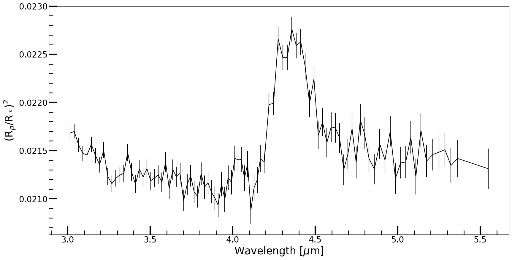
f=jpi.plot_errorbar(wlgrid_center, rprs_data2,e_rprs2, plot_type='matplotlib',
                   plot_kwargs={'ylabel':r'(R$_p$/R$_*$)$^2$'})#plot_type='bokeh' also available
#jpi.show(f) #if using bokeh (note if using bokeh need those key words (e.g. y_axis_label instead of ylabel))

../../_images/notebooks_fitdata_GridSearch_4_0.png

Add Available Grids to Test¶

First step will be to load your first grid into the GridFitter class. You can do this easily by supplying the function a directory location, and grid name (grid_name).

The only purpose of grid_name is in case you add more grids to your GridFitter function, it will be easy to keep track of what parameters go with what grid.

[4]:

grid_name = "picaso_cld_free"
location = os.path.join(model_dir,"RCTE_cloud_free")
fitter = lyz.GridFitter(grid_name,location, verbose=True)

Total number of models in grid is 192
For tint in planet_params grid is: [100. 200. 300.]
For heat_redis in planet_params grid is: [0.4 0.5]
For mh in planet_params grid is: [  0.1     0.316   1.      3.162  10.     31.623  50.119 100.   ]
For cto in planet_params grid is: [0.229 0.458 0.687 0.916]

This shows you what parameters the grid was created over

[5]:

fitter.grid_params['picaso_cld_free']['planet_params'].keys()

[5]:

dict_keys(['tint', 'heat_redis', 'mh', 'cto'])

[6]:

location = os.path.join(model_dir,"RCTE_cloudy")
fitter.add_grid('picaso_cldy', location)#

Total number of models in grid is 3840
For tint in planet_params grid is: [100. 200. 300.]
For heat_redis in planet_params grid is: [0.4 0.5]
For logkzz in planet_params grid is: [ 5.  7.  9. 11.]
For mh in planet_params grid is: [  0.1     0.316   1.      3.162  10.     31.623  50.119 100.   ]
For cto in planet_params grid is: [0.229 0.458 0.687 0.916]
For fsed in cld_params grid is: [ 0.6  1.   3.   6.  10. ]

Explore the parameters of the grid¶

You can see what grids you have loaded

[7]:

fitter.grids #what grids exist

[7]:

['picaso_cld_free', 'picaso_cldy']

You can also see what the top level information about your grid is

[8]:

fitter.overview['picaso_cld_free']#top level info from the attrs

[8]:

{'planet_params': {'rp': 1.279,
  'mp': 0.28,
  'tint': array([100., 200., 300.]),
  'heat_redis': array([0.4, 0.5]),
  'p_reference': 10.0,
  'logkzz': 'Not used in grid.',
  'mh': array([  0.1  ,   0.316,   1.   ,   3.162,  10.   ,  31.623,  50.119,
         100.   ]),
  'cto': array([0.229, 0.458, 0.687, 0.916]),
  'p_quench': 'Not used in grid.',
  'rainout': 'Not used in grid.',
  'teff': nan,
  'logg': nan,
  'm_length': nan},
 'stellar_params': {'rs': 0.932,
  'logg': 4.38933,
  'steff': 5326.6,
  'feh': -0.03,
  'ms': 0.913},
 'cld_params': {'opd': 'Not used in grid.',
  'ssa': 'Not used in grid.',
  'asy': 'Not used in grid.',
  'p_cloud': 'Not used in grid.',
  'haze_eff': nan,
  'fsed': 'Not used in grid.'},
 'num_params': 4}

The full list of planet parameters can also be cross referenced against the full list of file names so you can easily plot of different models.

[9]:

print(fitter.grid_params['picaso_cld_free']['planet_params']['tint'][0],
#this full list can be cross referened against the file list
fitter.list_of_files['picaso_cld_free'][0])
#in this case we can verify against the filename

100.0 /data2/models/WASP-39B/xarray/RCTE_cloud_free/profile_eq_planet_100_grav_4.5_mh_+1.0_CO_2.0_sm_0.0486_v_0.4_.nc

Add Datasets to Explore¶

Though the models are interesting, what we are really after is which is most representative of the data. So now let’s add some datasets to explore.

[10]:

fitter.add_data('firefly',wlgrid_center, wlgrid_width, rprs_data2, e_rprs2)

Compute \(\chi_{red}^2\)/N and Retrieve Single Best Fit¶

In this analysis we used the reduced chi sq per data point as a metric to fit the grid. This fitter function will go through your whole grid and compute cross reference the chi sq compared to your data.

[11]:

fitter.fit_grid('picaso_cld_free','firefly')
fitter.fit_grid('picaso_cldy','firefly')

Now that we have accumulated results let’s turn this into a dictionary to easily see what we’ve done

[12]:

out = fitter.as_dict()#allows you to easily grab data
out.keys()

[12]:

dict_keys(['list_of_files', 'spectra_w_offset', 'rank_order', 'grid_params', 'offsets', 'chi_sqs', 'posteriors'])

We are most interested in the models with the best reduced chi sq. We can use our ranked order to get the models that best fit the data.

[13]:

### Use rank order to get the top best fit or other parameters
#top 5 best fit models metallicities for the cloud free grid
print("cld free",np.array(out['grid_params']['picaso_cld_free']['planet_params']['mh']
        )[out['rank_order']['picaso_cld_free']['firefly']][0:5])

#top 5 best fit models metallicities for the cloudy grid
print("cldy",np.array(out['grid_params']['picaso_cldy']['planet_params']['mh']
        )[out['rank_order']['picaso_cldy']['firefly']][0:5])

cld free [100. 100. 100. 100. 100.]
cldy [ 3.162 10.    10.    10.    10.   ]

Interesting! We are already seeing interesting information. Without clouds our model predicts higher metallicity than when we add clouds. Let’s look at the associated chi square values.

[14]:

#top 5 best fit chi sqs for the cloud free grid
print("cld free", np.array(out['chi_sqs']['picaso_cld_free']['firefly']
        )[out['rank_order']['picaso_cld_free']['firefly']][0:5])

#top 5 best fit chi sq for the cloudy grid
print("cldy", np.array(out['chi_sqs']['picaso_cldy']['firefly']
        )[out['rank_order']['picaso_cldy']['firefly']][0:5])

cld free [1.91987567 1.92849109 1.9556125  2.00119925 2.01856747]
cldy [1.32818737 1.37253841 1.37564302 1.39244227 1.39555045]

The cloudy grid is giving lower chi square giving us clues that this planet likely has clouds affecting the spectrum.

Analyze Single Best Fits¶

Let’s analyze the single best fits in order to compare the spectrum with the data

[15]:

fig,ax = fitter.plot_best_fit(['picaso_cld_free','picaso_cldy'],'firefly')

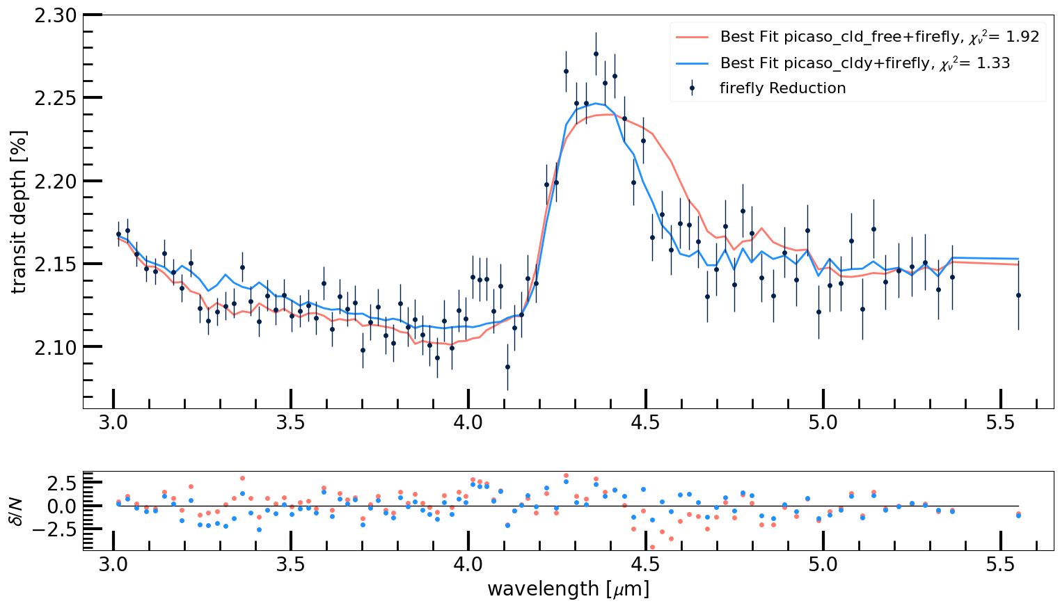
../../_images/notebooks_fitdata_GridSearch_30_0.png

By-eye, our cloudy grid is giving a much better representation of the data. Let’s look at what physical parameters are associated with this.

[16]:

best_fit = fitter.print_best_fit('picaso_cldy','firefly')

tint=100.0
heat_redis=0.5
logkzz=9.0
mh=3.162
cto=0.458
fsed=0.6

You can see these same parameters reported in original Nature paper: https://arxiv.org/pdf/2208.11692.pdf

Estimated Posteriors¶

It is also helpful to get an idea of what the probability is for each grid parameter in your model. This will give you a better representation of degeneracies that exist with your data and each of your physical parameters.

[17]:

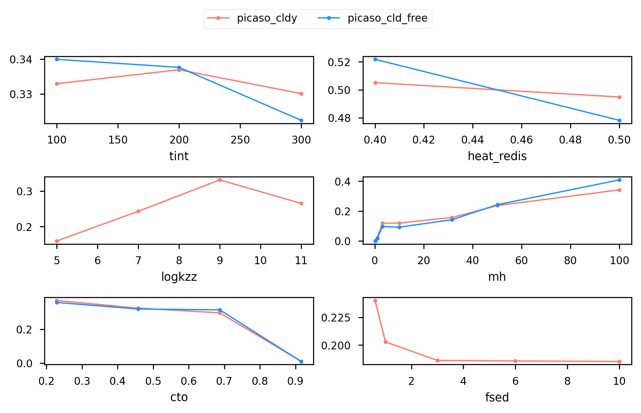
posterior_chance_dict, fig = fitter.plot_chi_posteriors(['picaso_cldy', 'picaso_cld_free'],
                                                        'firefly', max_row=3, max_col=2, input_parameters='all')

../../_images/notebooks_fitdata_GridSearch_35_0.png

[18]:

posterior_chance_dict

[18]:

{'picaso_cldy': {'tint': {'100.0'},
  'heat_redis': {'0.4'},
  'logkzz': {'9.0'},
  'mh': {'100.0'},
  'cto': {'0.229'},
  'fsed': {'0.6'}},
 'picaso_cld_free': {'tint': {'100.0'},
  'heat_redis': {'0.4'},
  'logkzz': {'9.0'},
  'mh': {'100.0'},
  'cto': {'0.229'},
  'fsed': {'0.6'}}}

What can you take away from this plot? 1. Cloudy models reduce the number of models that can be fit to the data with high metallicity 2. Internal temperature cannot be constrained by the data 3. C/O ratios greater than ~0.8 can be ruled out by the data

Interpret Best Fit¶

Now that we are happy with the best-fitting model, we can load in that data and post process some plots in order to gain better understanding of our results.

We can use PICASO’s xarray loader to quickly load in one of our models.

[19]:

#grab top model
top_model_file  = np.array(out['list_of_files']['picaso_cldy']
        )[out['rank_order']['picaso_cldy']['firefly']][0]

xr_usr = jdi.xr.load_dataset(top_model_file)
#take a look at the Xarray file
xr_usr

[20]:

opa = jdi.opannection(wave_range=[3,5])
case = jdi.input_xarray(xr_usr, opa)
#if you need to rerun your spectrum
#out = case.spectrum(opa,calculation='transmisson')

See Contribution From Each Molecule¶

One of the most common plots that was also used in the original paper is the “leave one out” method to see how each molecule is affecting our spectrum.

[21]:

#copy atmo before modifying and rerunning picaso
og_atmo = jdi.copy.deepcopy(case.inputs['atmosphere']['profile'])
#atmo
w,f,l =[],[],[]
for iex in ['CH4','H2O','CO2',None]:
    case.atmosphere(df = og_atmo,exclude_mol=iex, delim_whitespace=True)
    df= case.spectrum(opa, full_output=True,calculation='transmission') #note the new last key
    wno, rprs2  = df['wavenumber'] , df['transit_depth']
    wno, rprs2 = jdi.mean_regrid(wno, rprs2, R=150)
    w +=[wno]
    f+=[rprs2]
    if iex==None:
        leg='all'
    else:
        leg = f'No {iex}'
    l+=[leg]
jpi.show(jpi.spectrum(w,f,legend=l))

Quantify Molecular Detection using Guassian Fitting¶

For very gaussian shaped molecules (like CO2 in this case), we can use a simple Gaussian fitting technique to quantify the significance of our detection. Note this ONLY works in cases where the shape of the molecule is gaussian with a single peak and well-shaped wings.

[22]:

#grab file to test
top_model_file  = np.array(out['list_of_files']['picaso_cldy']
        )[out['rank_order']['picaso_cldy']['firefly']][0]

min_wave = 3 #min wave to search for gauss peak
max_wave = 5 #max wave to search for gauss peak
out = lyz.detection_test(fitter,'CO2',min_wave,max_wave,'picaso_cldy','firefly',
                     top_model_file,
                     #opa_kwargs={wave_range=[]}#this is where you input arguments for opannection
                     plot=True)

8676it [00:16, 535.41it/s, +500 | bound: 26 | nc: 1 | ncall: 37091 | eff(%): 25.077 | loglstar:   -inf < -77.771 <    inf | logz: -94.391 +/-  0.182 | dlogz:  0.001 >  0.509]
2562it [00:06, 389.20it/s, +500 | bound: 2 | nc: 1 | ncall: 19385 | eff(%): 16.214 | loglstar:   -inf < -466.966 <    inf | logz: -471.182 +/-  0.073 | dlogz:  0.001 >  0.509]

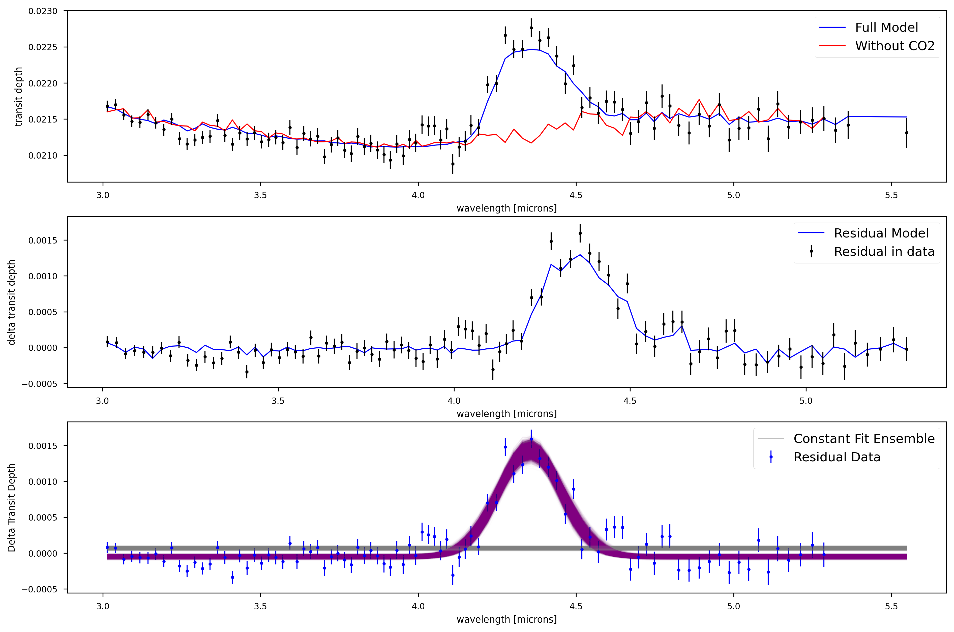
../../_images/notebooks_fitdata_GridSearch_44_1.png

By comparing the line fit to the single Gaussian fit, we can use the methodology of Trotta 2008 to get out a sigma detection significance. In this case we can see that the single gaussian fit is preferred over the line model at 26 sigma.

[23]:

out['sigma_single_v_line']

[23]:

27.575580879765575