JWST Tutorial
Here you will learn how to:
set planet properties
set stellar properties
run default instrument modes
adjust instrument modes
run pandexo
import warnings
warnings.filterwarnings('ignore')
import pandexo.engine.justdoit as jdi # THIS IS THE HOLY GRAIL OF PANDEXO
import numpy as np
import os
#pip install pandexo.engine --upgrade
Setting up a run
To start, load in a blank exoplanet dictionary with empty keys. You will fill these out for yourself in the next step.
exo_dict = jdi.load_exo_dict()
print(exo_dict.keys())
#print(exo_dict['star']['w_unit'])
Edit exoplanet observation inputs
Editting each keys are annoying. But, do this carefully or it could result in nonsense runs
exo_dict['observation']['sat_level'] = 80    #saturation level in percent of full well
exo_dict['observation']['sat_unit'] = '%'
exo_dict['observation']['noccultations'] = 2 #number of transits
exo_dict['observation']['R'] = None          #fixed binning. I usually suggest ZERO binning.. you can always bin later
                                             #without having to redo the calcualtion
exo_dict['observation']['baseline_unit'] = 'total'  #Defines how you specify out of transit observing time
                                                    #'frac' : fraction of time in transit versus out = in/out
                                                    #'total' : total observing time (seconds)
exo_dict['observation']['baseline'] = 4.0*60.0*60.0 #in accordance with what was specified above (total observing time)

exo_dict['observation']['noise_floor'] = 0   #this can be a fixed level or it can be a filepath
                                             #to a wavelength dependent noise floor solution (units are ppm)
Edit exoplanet host star inputs
Note… If you select ‘phoenix’ you do not have to provide a starpath, w_unit or f_unit, but you do have to provide a temp, metal and logg. If you select ‘user’ you do not need to provide a temp, metal and logg, but you do need to provide units and starpath.
exo_dict['star']['type'] = 'phoenix'        #phoenix or user (if you have your own)
exo_dict['star']['mag'] = 8.0               #magnitude of the system
exo_dict['star']['ref_wave'] = 1.25         #For J mag = 1.25, H = 1.6, K =2.22.. etc (all in micron)
exo_dict['star']['temp'] = 5500             #in K
exo_dict['star']['metal'] = 0.0             # as log Fe/H
exo_dict['star']['logg'] = 4.0              #log surface gravity cgs
Edit exoplanet inputs using one of three options
user specified
constant value
select from grid
1) Edit exoplanet planet inputs if using your own model
exo_dict['planet']['type'] ='user'                       #tells pandexo you are uploading your own spectrum
exo_dict['planet']['exopath'] = 'wasp12b.txt'
exo_dict['planet']['w_unit'] = 'cm'                      #other options include "um","nm" ,"Angs", "sec" (for phase curves)
exo_dict['planet']['f_unit'] = 'rp^2/r*^2'               #other options are 'fp/f*'
exo_dict['planet']['transit_duration'] = 2.0*60.0*60.0   #transit duration
exo_dict['planet']['td_unit'] = 's'                      #Any unit of time in accordance with astropy.units can be added
2) Users can also add in a constant temperature or a constant transit depth
exo_dict['planet']['type'] = 'constant'                  #tells pandexo you want a fixed transit depth
exo_dict['planet']['transit_duration'] = 2.0*60.0*60.0   #transit duration
exo_dict['planet']['td_unit'] = 's'
exo_dict['planet']['radius'] = 1
exo_dict['planet']['r_unit'] = 'R_jup'            #Any unit of distance in accordance with astropy.units can be added here
exo_dict['star']['radius'] = 1
exo_dict['star']['r_unit'] = 'R_sun'              #Same deal with astropy.units here
exo_dict['planet']['f_unit'] = 'rp^2/r*^2'        #this is what you would do for primary transit

#ORRRRR....
#if you wanted to instead to secondary transit at constant temperature
exo_dict['planet']['f_unit'] = 'fp/f*'
exo_dict['planet']['temp'] = 1000
3) Select from grid
NOTE: Currently only the fortney grid for hot Jupiters from Fortney+2010 is supported. Holler though, if you want another grid supported
exo_dict['planet']['type'] = 'grid'                #tells pandexo you want to pull from the grid
exo_dict['planet']['temp'] = 1000                 #grid: 500, 750, 1000, 1250, 1500, 1750, 2000, 2250, 2500
exo_dict['planet']['chem'] = 'noTiO'              #options: 'noTiO' and 'eqchem', noTiO is chemical eq. without TiO
exo_dict['planet']['cloud'] = 'ray10'               #options: nothing: '0',
#                                                   Weak, medium, strong scattering: ray10,ray100, ray1000
#                                                   Weak, medium, strong cloud: flat1,flat10, flat100
exo_dict['planet']['mass'] = 1
exo_dict['planet']['m_unit'] = 'M_jup'            #Any unit of mass in accordance with astropy.units can be added here
exo_dict['planet']['radius'] = 1
exo_dict['planet']['r_unit'] = 'R_jup'            #Any unit of distance in accordance with astropy.units can be added here
exo_dict['star']['radius'] = 1
exo_dict['star']['r_unit'] = 'R_sun'              #Same deal with astropy.units here
exo_dict['planet']['transit_duration'] = 2.0*60.0*60.0   #transit duration
exo_dict['planet']['td_unit'] = 's'
Load in instrument dictionary (OPTIONAL)
Step 2 is optional because PandExo has the functionality to automatically load in instrument dictionaries. Skip this if you plan on observing with one of the following and want to use the subarray with the smallest frame time and the readout mode with 1 frame/1 group (standard): - NIRCam F444W - NIRSpec Prism - NIRSpec G395M - NIRSpec G395H - NIRSpec G235H - NIRSpec G235M - NIRCam F322W - NIRSpec G140M - NIRSpec G140H - MIRI LRS - NIRISS SOSS
#jdi.print_instruments()
result = jdi.run_pandexo(exo_dict,['NIRCam F322W2'])
inst_dict = jdi.load_mode_dict('NIRSpec G140H')

#loading in instrument dictionaries allow you to personalize some of
#the fields that are predefined in the templates. The templates have
#the subbarays with the lowest frame times and the readmodes with 1 frame per group.
#if that is not what you want. change these fields

#Try printing this out to get a feel for how it is structured:

print(inst_dict['configuration'])
#Another way to display this is to print out the keys
inst_dict.keys()
Don’t know what instrument options there are?
print("SUBARRAYS")
print(jdi.subarrays('nirspec'))

print("FILTERS")
print(jdi.filters('nircam'))

print("DISPERSERS")
print(jdi.dispersers('nirspec'))
#you can try personalizing some of these fields

inst_dict["configuration"]["detector"]["ngroup"] = 'optimize'   #running "optimize" will select the maximum
                                                                #possible groups before saturation.
                                                                #You can also write in any integer between 2-65536

inst_dict["configuration"]["detector"]["subarray"] = 'substrip256'   #change the subbaray
Adjusting the Background Level
You may want to think about adjusting the background level of your observation, based on the position of your target. PandExo two options and three levels for the position:
eclipticorminzodilow,medium,high
inst_dict['background'] = 'ecliptic'
inst_dict['background_level'] = 'high'
Running NIRISS SOSS Order 2
PandExo only will extract a single order at a time. By default, it is set to extract Order 1. Below you can see how to extract the second order.
NOTE! Users should be careful with this calculation. Saturation will
be limited by the first order. Therefore, I suggest running one
calculation with ngroup='optmize' for Order 1. This will give you an
idea of a good number of groups to use. Then, you can use that in this
order 2 calculation.
inst_dict = jdi.load_mode_dict('NIRISS SOSS')
inst_dict['strategy']['order'] = 2
inst_dict['configuration']['detector']['subarray'] = 'substrip256'
ngroup_from_order1_run = 2
inst_dict["configuration"]["detector"]["ngroup"] = ngroup_from_order1_run
Running PandExo
You have four options for running PandExo. All of them are accessed through attribute jdi.run_pandexo. See examples below.
jdi.run_pandexo(exo, inst, param_space = 0, param_range = 0,save_file = True, output_path=os.getcwd(), output_file = '')
Option 1- Run single instrument mode, single planet
If you forget which instruments are available run jdi.print_isntruments() and pick one
jdi.print_instruments()
result = jdi.run_pandexo(exo_dict,['NIRCam F322W2'])
Option 2- Run single instrument mode (with user dict), single planet
This is the same thing as option 1 but instead of feeding it a list of keys, you can feed it a instrument dictionary (this is for users who wanted to simulate something NOT pre defined within pandexo)
inst_dict = jdi.load_mode_dict('NIRSpec G140H')
#personalize subarray
inst_dict["configuration"]["detector"]["subarray"] = 'sub2048'
result = jdi.run_pandexo(exo_dict, inst_dict)
Option 3- Run several modes, single planet
Use several modes from print_isntruments() options.
#choose select
result = jdi.run_pandexo(exo_dict,['NIRSpec G140M','NIRSpec G235M','NIRSpec G395M'],
               output_file='three_nirspec_modes.p')
#run all
#result = jdi.run_pandexo(exo_dict, ['RUN ALL'], save_file = False)
Option 4- Run single mode, several planet cases
Use a single modes from print_isntruments() options. But explore parameter space with respect to any parameter in the exo dict. The example below shows how to loop over several planet models
You can loop through anything in the exoplanet dictionary. It will be planet, star or observation followed by whatever you want to loop through in that set.
i.e. planet+exopath, star+temp, star+metal, star+logg, observation+sat_level.. etc
#looping over different exoplanet models
jdi.run_pandexo(exo_dict, ['NIRCam F444W'], param_space = 'planet+exopath',
                param_range = os.listdir('/path/to/location/of/models'),
               output_path = '/path/to/output/simulations')

#looping over different stellar temperatures
jdi.run_pandexo(exo_dict, ['NIRCam F444W'], param_space = 'star+temp',
                param_range = np.linspace(5000,8000,2),
               output_path = '/path/to/output/simulations')

#looping over different saturation levels
jdi.run_pandexo(exo_dict, ['NIRCam F444W'], param_space = 'observation+sat_level',
                param_range = np.linspace(.5,1,5),
               output_path = '/path/to/output/simulations')
Running PandExo GUI
The same interface that is available online is also available for use on your machine. Using the GUI is very simple and good alternative if editing the input dictionaries is confusing.
start_pandexo
Then open up your favorite internet browser and go to: http://localhost:1111
Analyzing Output
There are pre computed functions for analyzing most common outputs. You can also explore the dictionary structure yourself.
import pandexo.engine.justplotit as jpi
import pickle as pk
Plot 1D Data with Errorbars
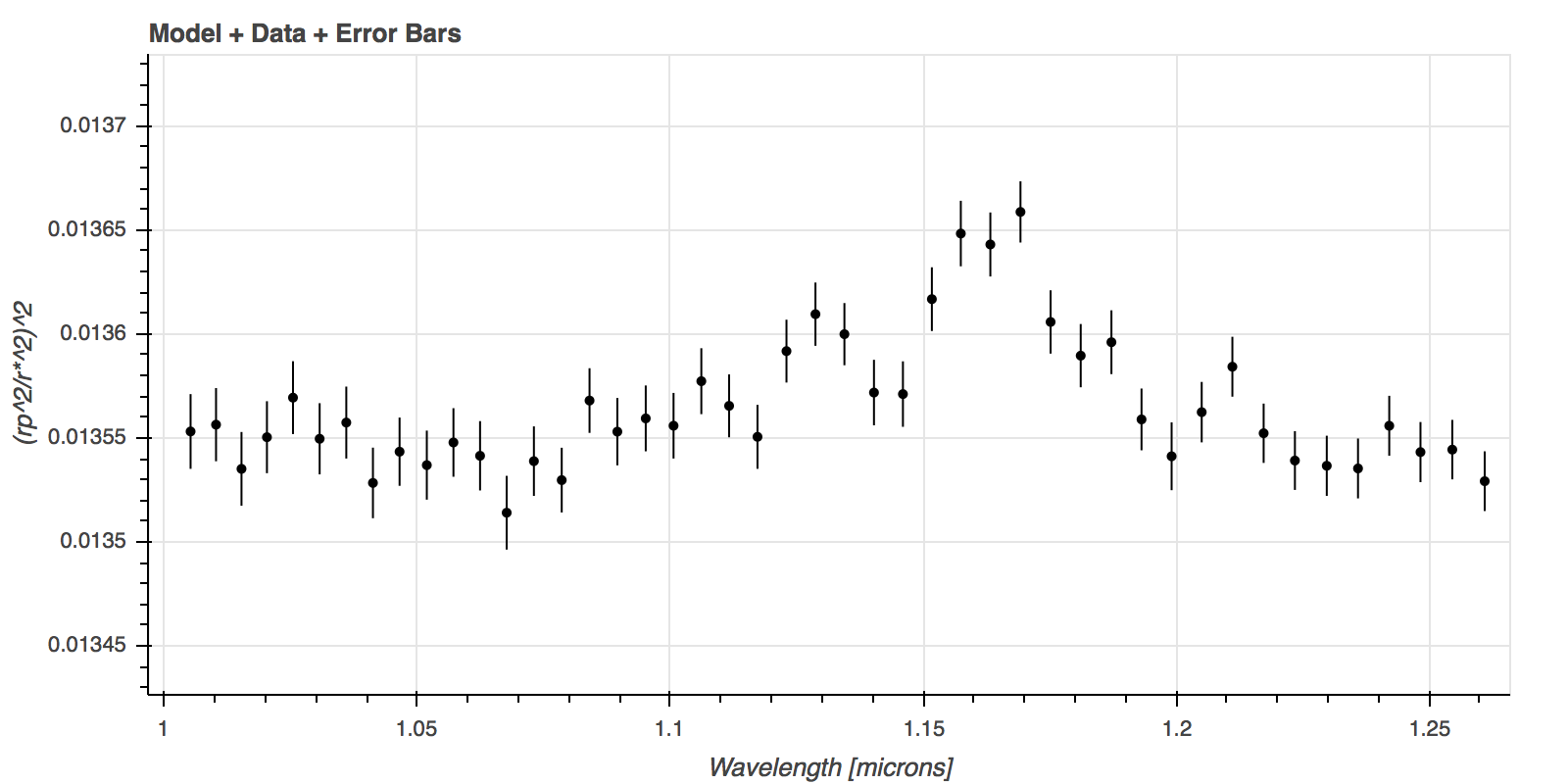
Multiple plotting options exist within jwst_1d_spec
Plot a single run
#load in output from run
out = pk.load(open('singlerun.p','r'))
#for a single run
x,y, e = jpi.jwst_1d_spec(out, R=100, num_tran=10, model=False, x_range=[.8,1.28])

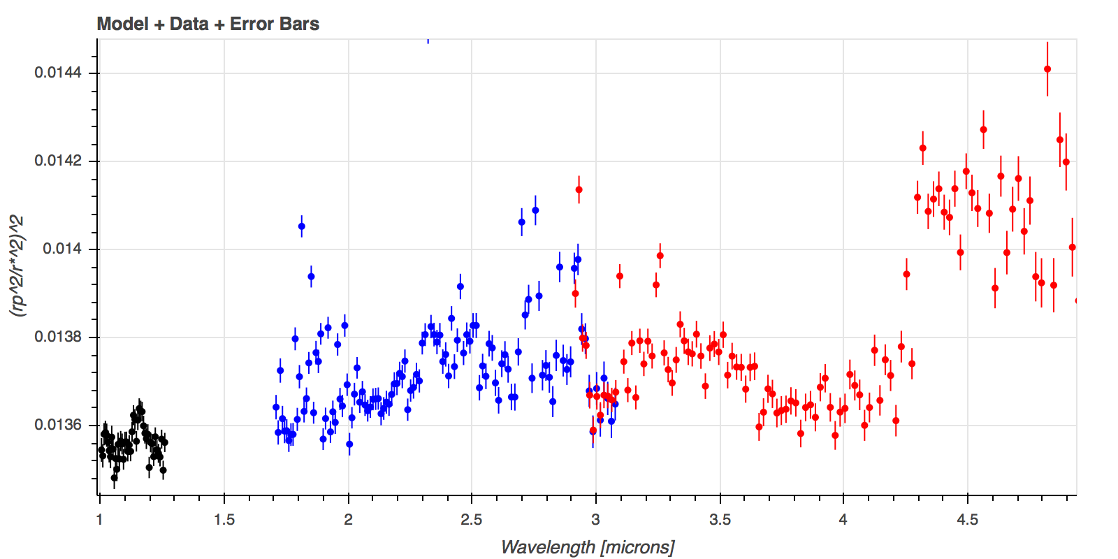
Plot several runs from parameters space run
#load in output from multiple runs
multi = pk.load(open('three_nirspec_modes.p','r'))

#get into list format
list_multi = [multi[0]['NIRSpec G140M'], multi[1]['NIRSpec G235M'], multi[2]['NIRSpec G395M']]

x,y,e = jpi.jwst_1d_spec(list_multi, R=100, model=False, x_range=[1,5])

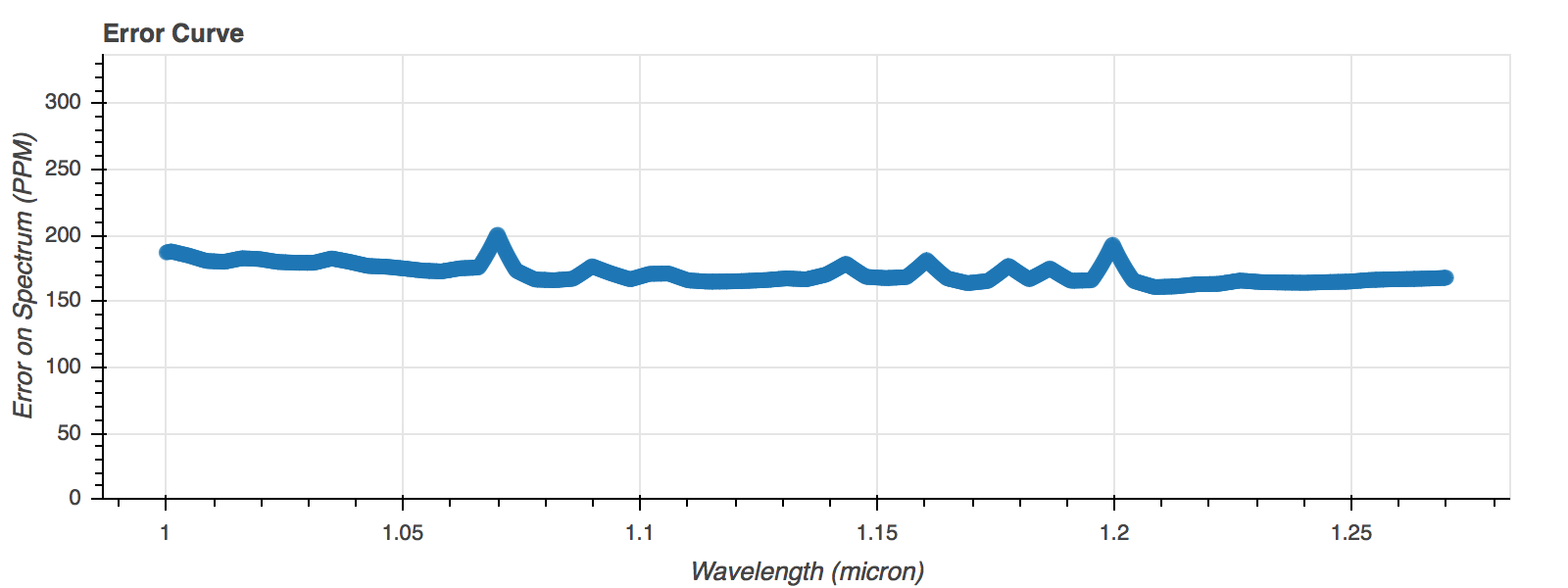
Plot Noise & More
Several functions exist to plot various outputs.
See also jwst_1d_bkg, jwst_1d_snr, jwst_1d_flux,
x,y = jpi.jwst_noise(out)

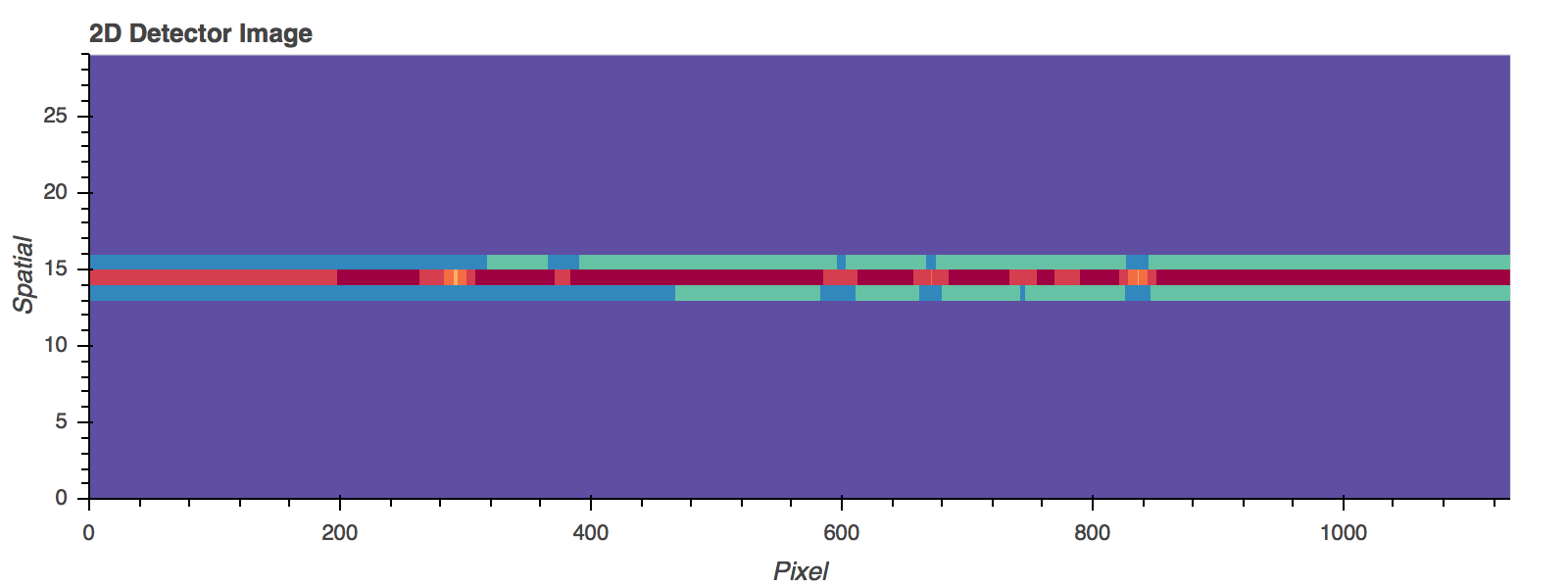
Plot 2D Detector Profile
See also jwst_2d_sat to plot saturation profile
data = jpi.jwst_2d_det(out)
