# ---
# jupyter:
# jupytext:
# custom_cell_magics: kql
# text_representation:
# extension: .py
# format_name: percent
# format_version: '1.3'
# jupytext_version: 1.11.2
# kernelspec:
# display_name: pic312
# language: python
# name: python3
# ---
# %% [markdown]
# # Initial Setup
#
# This tutorial has two big package dependencies: 1) `PandExo`, 2) `PICASO`
#
# Each of these depend on pretty hefty reference data packages that include things such as opacities, chemistry, _JWST_ reference data.
#
# ## Download Files and Install Extra Packages beyond PICASO
#
# This is a lot of data so I recommend downloading it early, and ensuring you have enough storage space. Make sure you've gone through the quickstart and have checked your environment. Note, this tutorial requires an additional isntall of PandExo, which is completely separate from PICASO. You will need to install this on your own
#
# 1. Install PandExo (separate package with separate installation instructions)
#
#
# ### Make sure we have the right PICASO data
#
# 1. Are you a student and want to quickly run this without going through full PICASO data install setup? **PROCEED TO A do not edit B**
#
# 2. Have you already installed picaso, set reference variables, and have an understanding of how to get new data products associated with PICASO? **PROCEED TO edit B.**
# %%
import picaso.data as d
#uncomment and set path if you need to do this in the tutorial
#picaso_refdata = '/data/test/tutorial/picaso-lite-reference' #change to where you want this to live
"""
A) Uncomment if you need the picaso-lite data
"""
#d.os.environ['picaso_refdata'] = picaso_refdata
#if you do not yet have the picaso reference data complete this step below
#d.get_data(category_download='picaso-lite', target_download='tutorial_sagan23',final_destination_dir=picaso_refdata)
"""
B) Edit accordingly if needed (no need to edit if completed "A" above)
"""
#uncomment picaso ref data, if need to set it
#d.os.environ['picaso_refdata'] = picaso_refdata
# uncomment stellar data environment
#d.os.environ['PYSYN_CDBS'] = d.os.path.join(d.os.environ['picaso_refdata'],'stellar_grids')
#lets check your environment
d.check_environ()
#dont have the data? return to the step A above to use the get_data function
# %%
# STEP 1: PandExo Reference Data if you have not already
d.os.environ['pandeia_refdata'] = '/data/pandexo/pandeia_data-2025.7-jwst'
# %%
import warnings
warnings.filterwarnings("ignore")
#python tools
import requests
import numpy as np
import pandas as pd
from bokeh.plotting import figure, show
import bokeh.palettes as color
from bokeh.io import output_notebook
from bokeh.layouts import row, column
output_notebook()
#double check that you have loaded BokehJS 2.1.1
# %% [markdown]
# # What accuracy in planet properties do I need?
# %% [markdown]
# ## Using `Exoplanet Archive API` to Query Confirmed Targets
#
# We can query from Exoplanet Archive to get a list of targets. Once we have all the targets we will have to narrow down the sample to only those that have suitable planet properties.
# %%
planets_df = pd.read_csv('https://exoplanetarchive.ipac.caltech.edu/TAP/sync?query=select+*+from+PSCompPars&format=csv')
# %%
# convert to float when possible
for i in planets_df.columns:
planets_df[i] = planets_df[i].astype(float,errors='ignore')
# %%
#voila
planets_df.head()
# %% [markdown]
# ### Trouble finding what you are looking for?
# %%
#easy way to search through dataframe with many keys
[i for i in planets_df.keys() if 'mass' in i]
# %% [markdown]
# ### Get rid of everything without a mass
# %%
#let's only grab targets with masses and errors
pl_mass_err = planets_df.loc[:,['pl_bmassjerr1', 'pl_bmassj']].astype(float)
pl_mass_err = pl_mass_err.dropna()
# %% [markdown]
# Percentage of planets in NexSci database with masses
# %%
100*pl_mass_err.shape[0]/planets_df.shape[0]
# %% [markdown]
# Now let's get an idea of what those mass errors are
# %%
pl_mass_fig = figure(x_axis_type='log', width=550, height=400, x_axis_label='Mj',
y_axis_label='Mass Uncertainty',y_range=[0,150],x_range=[1e-3, 10])
pl_mass_fig.scatter(pl_mass_err['pl_bmassj'],
100*pl_mass_err['pl_bmassjerr1']/pl_mass_err['pl_bmassj'],
color='black', size=5, alpha=0.5)
pl_mass_fig.outline_line_color='black'
pl_mass_fig.outline_line_width=3
pl_mass_fig.xgrid.grid_line_alpha=0
show(pl_mass_fig)
# %% [markdown]
# We only want targets with mass precision better than ~20%.
#
# Let's also take only those targets that are brighter than J<12
# %%
#mass err less better than 20%
potential_props = pl_mass_err.loc[100*pl_mass_err['pl_bmassjerr1']/pl_mass_err['pl_bmassj']<20]
potential_props = planets_df.loc[pl_mass_err.index,:]
# %%
#brighter than 12
choose_from = potential_props.loc[potential_props['sy_jmag']<12]
# %%
choose_from.shape[0]
# %% [markdown]
# # What tools do I need? How do I use them?
#
# ## Use `PandExo` to run initial constant $(R_p/R_*)^2$ to determine approx precision
#
# Let's choose a single planet GJ 436 b as our example to evaluate observability.
#
# **Should'e already downloaded data**: We won't go through the details of installation and default data. The `conda` environment on here should have installed PandExo. In order for this to work you will need to download the [necessary default data](#download). You can also go to the [PandExo Installation Page](https://natashabatalha.github.io/PandExo/).
# %%
#check to make sure it's in our list of nicely constained masses
choose_from.head()
# %%
# load pandexo
import pandexo.engine.justdoit as jdi
import pandexo.engine.justplotit as jpi
import pandexo.engine.bintools as bi
# %%
planet_name = 'GJ 436 b'
GJ436b = jdi.load_exo_dict(planet_name=planet_name)
# %% [markdown]
# For this initial run, the only 2 parameters you need to edit are:
#
# 1. Saturation level within the `observation` key: This will determine how many groups can fit with in an integration. Let's keep this at 80% to be safe.
#
# 2. Change planet type to constant so that we don't have to input an atmospheric model yet.
# %%
GJ436b['planet']['type'] = 'constant'
GJ436b['planet']['f_unit'] = 'rp^2/r*^2'
# %%
GJ436b['observation']['sat_level'] = 80
GJ436b['observation']['sat_unit'] = '%'
# %% [markdown]
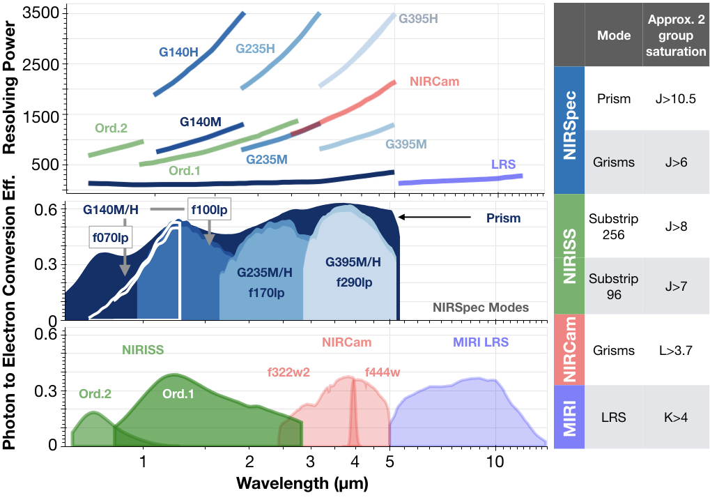
# Next pick an initial set of instrument modes. I usually pick one at least one from each of the 4 (NIRISS, NIRSpec, NIRCam, and MIRI).
#
#
#
# %%
to_run = ['NIRISS SOSS', 'NIRSpec G395H', 'NIRCam F444W','MIRI LRS']
result = jdi.run_pandexo(GJ436b, to_run)
# %% [markdown]
# ### What is the approximate precision achieved by each observing mode in a single transit at native resolution??
# %%
prec_fig = figure(x_axis_type='log',y_range=[0,400],
height=300, x_axis_label='Wavelength(Micron)',
y_axis_label='Spectra Precision per pix (ppm)')
for i, inst in enumerate(to_run):
x = result[i][inst]['FinalSpectrum']['wave']
e = result[i][inst]['FinalSpectrum']['error_w_floor']*1e6 #PPM UNITS!
prec_fig.line(x,e, line_width=4, color = color.Colorblind6[i],legend_label=inst)
prec_fig.legend.location='top_left'
prec_fig.outline_line_color='black'
prec_fig.outline_line_width=3
prec_fig.xgrid.grid_line_alpha=0
prec_fig.ygrid.grid_line_alpha=0
show(prec_fig)
# %% [markdown]
# ### What is the approximate precision achieved by each observing mode in a single transit at $R = 100$ ??
#
# %%
from bokeh.io import reset_output
prec_fig = figure(x_axis_type='log',y_range=[0,200],
height=300, x_axis_label='Wavelength(Micron)',
y_axis_label='Spectral Precision ber R=100 bin (ppm)')
ES = {} # let's use this to store the values
XS = {}
for i, inst in enumerate(to_run):
if 'MIRI' not in inst:#LRS is already at around 100, so let's keep it at native R
x,y,e = jpi.jwst_1d_spec(result[i][inst], plot=False, model=False, R=100)
# if you check out your plot below you'll see the noise budget blows up at the
# detector edges so I usually make a 5*median cut to get rid of the crap
x = x[0][np.where(e[0]<5*np.median(e[0]))]
e = e[0][np.where(e[0]<5*np.median(e[0]))]*1e6 #PPM UNITS!
#plot
prec_fig.line(x,e, line_width=4, color = color.Colorblind6[i],legend_label=inst)
else:
x = result[i][inst]['FinalSpectrum']['wave']
e = result[i][inst]['FinalSpectrum']['error_w_floor']
x = x[np.where(e<5*np.median(e))]
e = e[np.where(e<5*np.median(e))]*1e6 #PPM UNITS!
prec_fig.line(x,e, line_width=4, color = color.Colorblind6[i],legend_label=inst)
#lets save these for later
XS[inst] = x
ES[inst] = e
prec_fig.legend.location='top_left'
prec_fig.outline_line_color='black'
prec_fig.outline_line_width=3
prec_fig.xgrid.grid_line_alpha=0
prec_fig.ygrid.grid_line_alpha=0
reset_output()
output_notebook()
show(prec_fig)
# %% [markdown]
# ## Use `PICASO` to determine first guess atmospheric transmission signal
#
# From the `PandExo` exercise we've learned we can achieve approximately 30-50 ppm precision in a single transit. This is a great place to start. Now, we want to get a sense of _what this data precision gives us, scientifically speaking_.
#
# %% [markdown]
# Black box codes == there are many model parameters I am sweeping under the rug for the purposes of a clean and concise demo. With that cautionary note, we can proceed.
# %% [markdown]
# Unfortunately NexSci doesn't always have all the necessary planet properties. If you get an error below, that is likely why. For GJ 436b, this is the case. NexSci is missing two values : Stellar Fe/H and Stellar effective temperature. I have added those two as `kwargs` which I found from [Exo.MAST](https://exo.mast.stsci.edu/).
# %%
#load picaso
# load picaso
import picaso.justdoit as pj
import picaso.justplotit as pp
# %%
#load opacities
opas = pj.opannection(wave_range=[1,12]) #defined in code 1
#load planet in the same way as before
gj436_trans = pj.load_planet(choose_from.loc[choose_from['pl_name']==planet_name],
opas,
pl_eqt=667,st_metfe = 0.02, st_teff=3479)
# %% [markdown]
# ### The simplest, most optimistic case: Cloud free, Solar Metallicity, Solar C/O
#
#
# %%
#run picaso
log_mh = 0 #this is relative to solar, so 10**log_mh = 1xsolar
co = 0.55 # absolute solar value
gj436_trans.chemeq_visscher_2121(co,log_mh)
df_picaso = gj436_trans.spectrum(opas, calculation='transmission', full_output=True)
wno,cloud_free = pj.mean_regrid(df_picaso['wavenumber'], df_picaso['transit_depth'] , R=150)
# %%
spec = figure(x_axis_type='log', y_axis_label='Relative Transit Depth',
x_axis_label='Wavelength(micron)',
height=300)
#mean subtracting your spectrum will help you understand your spectrum in the context of
#your noise simulations above. Here I am choosing to normalize to 1 micron.
cf_norm = 1e6*(cloud_free - cloud_free[np.argmin(np.abs(1e4/wno-1))])
spec.line(1e4/wno, cf_norm , color='black',line_width=3)
for i, inst in enumerate(to_run):
fake_y =np.interp( XS[inst], 1e4/wno[::-1],cf_norm[::-1] )
spec.varea(x=XS[inst],
y1=fake_y + ES[inst],
y2=fake_y - ES[inst] , alpha=0.7, color=color.Colorblind6[i])
show(spec)
# %% [markdown]
# This looks GREAT but highly sus. A water amplitude of 200pm at 1.4 $\mu$m means we could've easily detected something with _Hubble_. Was that the case? For this particular planet, we can check `Exo.MAST` to see if there is a transmission spectrum available.
#
# ## Check `Exo.MAST` for available data so we can validate our assumptions
#
# First, let's check to see if a transmission spectrum exists. We can use `Exo.MAST`!
#
#
#
# __TO DO:__
#
# Navigate to `Exo.Mast`, search for GJ 436 b (or your planet) and you should see a tab on the figure for "transmission spectra". __Download the following file__.
# %%
IRL = pd.read_csv('/data2/observations/GJ-436b/HST/GJ436b_transmission_Knutson2014.txt', skiprows=8,
names = ['micron','dmicron','tdep','etdep'], sep=r'\s+')
# %% [markdown]
# Let's compare our real life data to what our optimistic `1xSolar` cloud free case is.
# %%
#as we go through this, let's save our models in a dictionary
all_models = {}
spec = figure(x_axis_type='log', y_axis_label='Relative Transit Depth',
x_axis_label='Wavelength(micron)',
height=300)
#normalizing your spectrum will help you understand your spectrum in the context of
#your noise simulations above
cf_norm = 1e6*(cloud_free - cloud_free[np.argmin(np.abs(1e4/wno-1))])
all_models['1x'] = cf_norm
all_models['um'] = 1e4/wno
spec.line(1e4/wno, cf_norm , color='black',line_width=3)
#again mean subtract from value at 1 micron so they line up, and convert to ppm
y =1e6*( IRL['tdep'] - IRL.iloc[(IRL['micron']-1).abs().argsort()[0],2])
#plot the data
pp.plot_errorbar( IRL['micron'], IRL['tdep']
, 1e6*IRL['etdep'] , spec,
#formatting
point_kwargs={'size':5,'color':'black'}, error_kwargs={'line_width':1,'color':'black'})
for i, inst in enumerate(to_run):
fake_y =np.interp( XS[inst], 1e4/wno[::-1],cf_norm[::-1] )
spec.varea(x=XS[inst],
y1=fake_y+ ES[inst],
y2=fake_y - ES[inst] , alpha=0.7, color=color.Colorblind6[i])
show(spec)
# %% [markdown]
# The model is way off.
#
# ### Proposals with 1xSolar cloud free claims are *not realistic*. What can we do to bolster our argument?
#
# The data precision required to rule a 1xSolar CF model is not high enough. Therefore, if one bases their total observing time on a 1xSolar model, they would be largely _under-asking_ for time. And, a TAC member might call out your proposal for having _over simplified_ your model results.
#
# Let's see what we can do to rectify this.
#
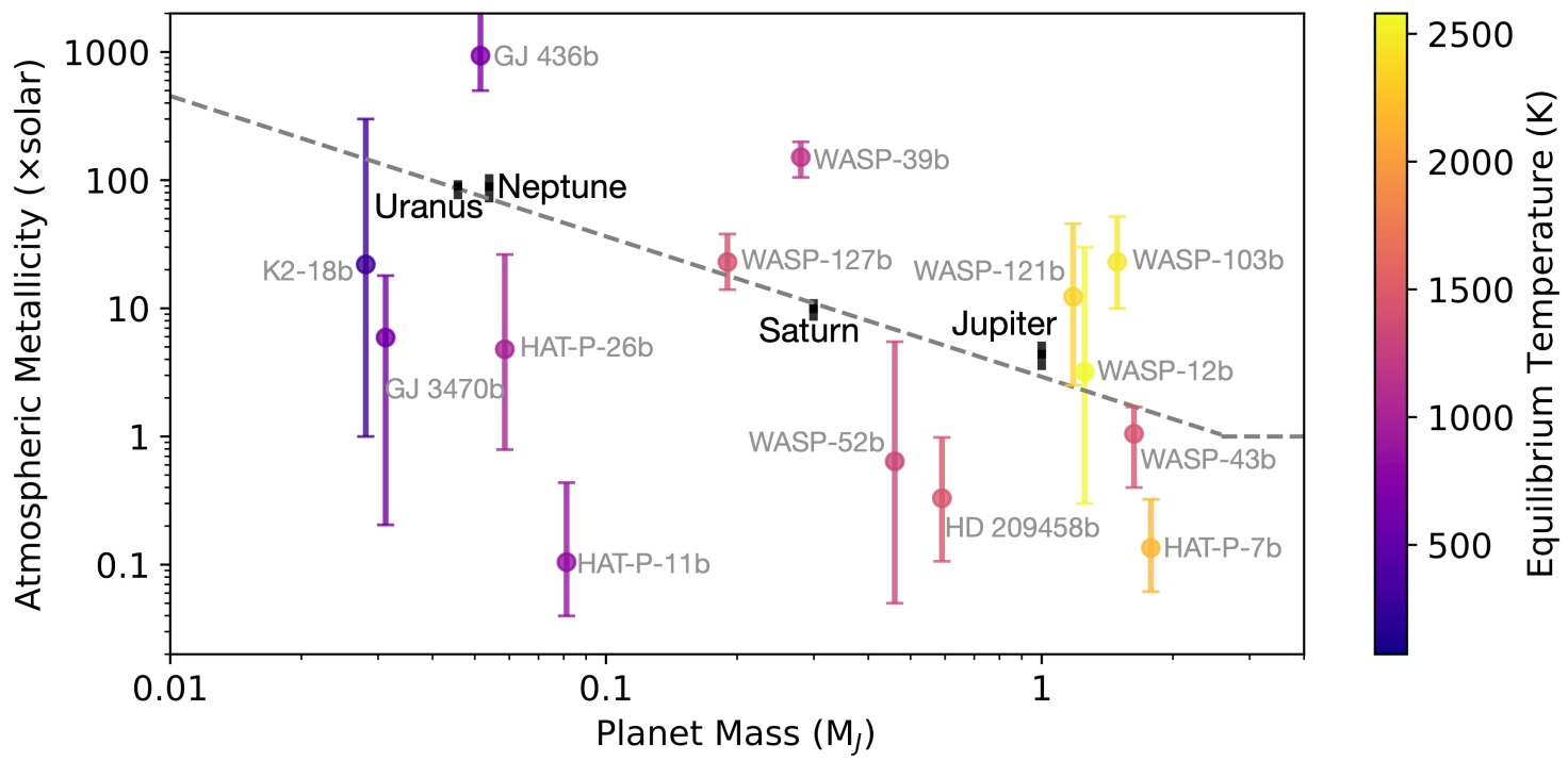
# ### Try following the Mass-M/H plot to get a more "realistic" prediction of what the of M/H should be
#
#
#
#
#
# Wakeford & Dalba 2020
#
#
#
# In this case we have an estimate for GJ 436b already. But, let's pretend we don't have that yet :)
#
# %%
#run picaso
log_mh = 2 #this is relative to solar, so 10**log_mh = 1xsolar
co = 0.55 # absolute solar value
gj436_trans.chemeq_visscher_2121(co,log_mh)
df_picaso = gj436_trans.spectrum(opas, calculation='transmission', full_output=True)
wno,cloud_free = pj.mean_regrid(df_picaso['wavenumber'], df_picaso['transit_depth'] , R=150)
# %% [markdown]
# Repeat the last exercise
# %%
#as we go through this, let's save our models
spec = figure(x_axis_type='log', y_axis_label='Relative Transit Depth',
x_axis_label='Wavelength(micron)',
height=300)
#normalizing your spectrum will help you understand your spectrum in the context of
#your noise simulations above
cf_norm = 1e6*(cloud_free - cloud_free[np.argmin(np.abs(1e4/wno-1))])
all_models['100x'] = cf_norm
spec.line(1e4/wno, cf_norm , color='black',line_width=3, legend_label='100xSolar')
spec.line(1e4/wno, all_models['1x'] , color='grey',line_width=3, legend_label='1xSolar')
#again mean subtract from value at 1 micron so they line up, and convert to ppm
y =1e6*( IRL['tdep'] - IRL.iloc[(IRL['micron']-1).abs().argsort()[0],2])
#plot the data
pp.plot_errorbar(IRL['micron'], IRL['tdep'] ,
1e6*IRL['etdep'] , spec,
#formatting
point_kwargs={'size':5,'color':'black'}, error_kwargs={'line_width':3,'color':'black'})
for i, inst in enumerate(to_run):
fake_y =np.interp( XS[inst], 1e4/wno[::-1],cf_norm[::-1] )
spec.varea(x=XS[inst],
y1=fake_y+ ES[inst],
y2=fake_y - ES[inst] , alpha=0.7, color=color.Colorblind6[i])
spec.legend.location='top_left'
show(spec)
# %% [markdown]
# Looks much better already. Unfortunately we aren't done quite yet.
#
# Let's revisit our first hierarchical question:
#
# 1. Can you detect an atmosphere?
#
# The answer seems obvious: **Of course!!!** Two important questions must be addressed:
#
# - At what level of significance?
# - What about clouds?
# - And other physical parameters? Temperature? C to O ratio?
#
# We will visit these questions in [Section 3: How can I prove observability](#section3).
#
# But first, let's run some first guess emission cases.
#
# ## Use `PICASO` to determine first guess atmospheric emission signal
#
# %%
planet_name = 'GJ 436 b'
# %%
#load opacities
opas = pj.opannection(wave_range=[1,12]) #defined in code 1
#load planet in the same way as before
gj436_emis = pj.load_planet(choose_from.loc[choose_from['pl_name']==planet_name],
opas,
pl_eqt=667,st_metfe = 0.02, st_teff=3479)
# right now picaso and chimera are using a PT profile parameterization
# I've made sure they are the same for the purposes of this demo
T = gj436_emis.inputs['atmosphere']['profile']['temperature'].values
P = gj436_emis.inputs['atmosphere']['profile']['pressure'].values
# %% [markdown]
# ### The simplest case: Cloud free, Solar Metallicity, Solar C/O
#
#
# For this demo we are going to use the same chemistry as chimera. Our little black body function contains the necessary function to grab the chemistry
# %%
all_emis = {}
# let's get the same chemistry as chimera for consistency
logMH = 0 #log relative to solar
CO = 0.55 #absolute solar value
#add in chemistry to picaso bundle
gj436_emis.chemeq_visscher_2121(CO, logMH)
#run picaso
df_picaso = gj436_emis.spectrum(opas, calculation='thermal', full_output=True)
wno, fpfs = pj.mean_regrid(df_picaso['wavenumber'], df_picaso['fpfs_thermal'] , R=150)
# %% [markdown]
# Plot with our error bars from `PandExo`
# %%
spec = figure(x_axis_type='log', y_axis_label='Eclipse Spectrum (Fplanet/Fstar)',
x_axis_label='Wavelength(micron)',
height=300)
all_emis['1xSolar'] = fpfs*1e6
spec.line(1e4/wno, fpfs*1e6 , color='black',line_width=3)
for i, inst in enumerate(to_run):
fake_y =np.interp( XS[inst], 1e4/wno[::-1],fpfs[::-1]*1e6 )
spec.varea(x=XS[inst],
y1=fake_y + ES[inst],
y2=fake_y - ES[inst] , alpha=0.7, color=color.Colorblind6[i])
show(spec)
# %% [markdown]
# Wahoo! Since we don't have similar transmission data for emission spectroscopy, let's use our initial 200xSolar guess that we had for transmission to see the difference.
# %%
logMH = 2 #log relative to solar
CO = 0.55 #absolute solar value
#add in chemistry to picaso bundle
gj436_emis.chemeq_visscher_2121(CO, logMH)
#run picaso
df_picaso = gj436_emis.spectrum(opas, calculation='thermal', full_output=True)
wno, fpfs = pj.mean_regrid(df_picaso['wavenumber'], df_picaso['fpfs_thermal'] , R=150)
spec = figure(x_axis_type='log', y_axis_label='Eclipse Spectrum (Fplanet/Fstar)',
x_axis_label='Wavelength(micron)',
height=300)
spec.line(1e4/wno, all_emis['1xSolar'], color='grey',line_width=3, legend_label='1xSolar')
all_emis['100xSolar'] = fpfs*1e6
spec.line(1e4/wno, fpfs*1e6 , color='black',line_width=3, legend_label='200xSolar')
for i, inst in enumerate(to_run):
fake_y =np.interp( XS[inst], 1e4/wno[::-1],fpfs[::-1]*1e6 )
spec.varea(x=XS[inst],
y1=fake_y + ES[inst],
y2=fake_y - ES[inst] , alpha=0.7, color=color.Colorblind6[i])
spec.legend.location='top_left'
show(spec)
# %% [markdown]
# ### My first guess transmission and/or emission signals look promising. What's next?
#
# Based on our initial 1x and 200x Solar models of transmission and emission, our simulations look great. So what is next?
#
# We have to take our analysis one step further to determine at what level of significance we can make these detections.
# %% [markdown]
#
# # How can I "prove" observability?
#
# The classic hierarchical science levels are:
#
# 1. Can you detect an atmosphere?
# 2. Can you detect a specific molecule?
# 3. Can you detect another physical process?
# 4. Can you _constrain_ a molecular abundance? A metallicity? A climate profile? An aerosol species?
#
# This section will walk you through steps to determine where you stand on in this hierarchy.
#
# ## Can an atmosphere be detected: Addressing cloud concerns and quantifying statistical significance in transmission
#
# First, let's expand our initial 1xSolar M/H case. Let's add a few cloud cases (e.g. no cloud, medium cloud, high cloud) and a few M/H cases and show first show how these relate to the expected data precision. Next we will discuss how to make these address our ability to detect (or not) each case.
# %%
logMHs = [0.5,1.0,1.5,2.0]
cloud_bottom = 1 #10 bars
cloud_thickness = [2,3,4,5] #these are log cross sections which
all_models_trans = {i:{} for i in logMHs}
fig = figure(height= 300,
x_axis_label='Wavelength(micron)',
y_axis_label='Relative Transit Depth (PPM)', x_axis_type='log')
colors = color.viridis(len(logMHs)*len(cloud_thickness))
ic = 0
for logMH in logMHs:
for log_dp in cloud_thickness:
CO = 0.55 #solar carbon to oxygen ratio
gj436_trans.chemeq_visscher_2121(CO, logMH)
#add in the cloud
gj436_trans.clouds(g0=[0.9], w0=[0.9], opd=[10], p=[cloud_bottom], dp=[log_dp])
#run picaso
df_picaso = gj436_trans.spectrum(opas, calculation='transmission', full_output=True)
wno, model = pj.mean_regrid(df_picaso['wavenumber'], df_picaso['transit_depth'] , R=150)
all_models_trans[logMH][log_dp] = 1e6*((model)- model[np.argmin(np.abs(1e4/wno-1))])
fig.line(1e4/wno, all_models_trans[logMH][log_dp] , color=colors[ic], line_width=3,
alpha=0.7,legend_label=str(logMH)+str(log_dp))
ic +=1
show(fig)
# %% [markdown]
# ### "Can an atmosphere be detected in transmission" usually translates to "can a $y=mx+b$ model be rejected"
# %%
fig = [figure(title = i, height= 250, width=300, x_axis_label='log Metallicity',
y_axis_label='log Cloud Cross Section', #y_range=[0,4],x_range=[0,2.5]
) for i in to_run]
#for our line model
from scipy.optimize import curve_fit
from scipy.stats.distributions import chi2
def line(x, a, b):
return a * x + b
all_ps = {i:[] for i in to_run}
for i, inst in enumerate(to_run):
for MH in logMHs:
for CLD in cloud_thickness:
y = all_models_trans[MH][CLD]
#wno is at lower res than our observation so we have to finagle them onto the same axis
binned_obs = bi.binning(XS[inst], XS[inst]*0, dy =ES[inst] ,newx=1e4/wno[::-1])
binned_model = pp.mean_regrid(wno, y, newx=1e4/binned_obs['bin_x'][::-1])[1]
#add random noise to your binned model which is now our "fake data"
fake_data = binned_model + np.random.randn(len(binned_obs['bin_dy']))*binned_obs['bin_dy']
#step 1) fit a line through each model
popt, pcov = curve_fit(line, binned_obs['bin_x'], fake_data, sigma =binned_obs['bin_dy'])
#now we have:
y_measured = fake_data
y_error = binned_obs['bin_dy']
y_line_model = line(binned_obs['bin_x'], popt[0], popt[1])
# .. and we can use tradition chi square p values to do some hypothesis testing
#compute chi square of each model
line_chi = np.sum((y_measured-y_line_model)**2/y_error**2)
p = chi2.sf(line_chi, len(y_measured) - 2)#2 because there are 2 free model params
all_ps[inst] += [[MH, CLD, p]]
#some crafy finagling to get a good color scheme
if p>0.05:
col = color.RdBu3[-1] #red if it cant be rejected
legend = 'Cannot Reject'
elif ((p<=0.05) & (p>=0.006)):
col = color.RdBu3[1] #white for medium/low rection
legend= 'Weak/Med Reject'
else:
col = color.RdBu3[0] #blue is strong rejection of line
legend='Strong Favor'
#hacked "heat map"
fig[i].scatter(MH, CLD, color = col, size=30,line_color='black',legend_label=legend,marker='square')
show(column(row(fig[0:2]), row(fig[2:4])))
# %% [markdown]
# From these figures we can immediately come to a few conclusions
#
# 1. NIRISS is most strongly impacted by clouds and has the least potential in being able to "detect an atmosphere" (e.g. reject a flat line hypothesis)
# 2. NIRSpec and NIRCam are best at rejecting the flat line
# 3. MIRI LRS struggles at rejecting flat line hypothesis
#
# You can _always_ create scenarios where an atmosphere is not detectable. For your proposal, it's only important to justify the level at which an atmosphere could be robustly detected.
# %% [markdown]
# ## Can an atmosphere be detected: Addressing unknown climate and quantifying statistical significance in emission
#
# First, let's expand our initial 1xSolar M/H case. In transmission we focused on M/H and cloud cross sectional strength. Although clouds will have an ultimate effect on the emission spectra, the first order affect is that of the pressure-temperature profile. So here, instead of running through M/H-cloud parameter space, we are going to run through a few M/H-temperature cases.
#
# **Theorists Caution:** To simplify this exercise we are parameterizing our pressure-temperature profiles. We urge groups to talk to their local theorist about the validity of this hack for your specific problem.
# %%
logMHs = [0.5,1.0,1.5,2.0]
DTs = [-100,0,100] #these are delta Kelvin amounts that we will use to perturb our PT profile
all_models_emis = {i:{} for i in logMHs}
fig = figure(height= 300,
x_axis_label='Wavelength(micron)',
y_axis_label='Fp/Fs (PPM)', x_axis_type='log')
colors = color.viridis(len(logMHs)*len(DTs))
ic = 0
for MH in logMHs:
for DT in DTs:
CO = 0.55 #solar carbon to oxygen ratio
#add in chemistry to picaso bundle T+DT, P
gj436_emis.inputs['atmosphere']['profile']['temperature'] = T + DT
gj436_emis.chemeq_visscher_2121(CO,MH)
#run picaso
df_picaso = gj436_emis.spectrum(opas, calculation='thermal', full_output=True)
wno_pic, fpfs = pj.mean_regrid(df_picaso['wavenumber'], df_picaso['fpfs_thermal'] , R=150)
#let's also save raw thermal flux (you'll see why next)
wno_pic, thermal = pj.mean_regrid(df_picaso['wavenumber'], df_picaso['thermal'] , R=150)
all_models_emis[MH][DT] = [fpfs*1e6,thermal]
fig.line(1e4/wno_pic, all_models_emis[MH][DT][0] , color=colors[ic], line_width=3,
alpha=0.7,legend_label=str(MH)+str(DT))
ic +=1
fig.legend.location='top_left'
show(fig)
# %% [markdown]
# ### "Can an atmosphere be detected in emission" usually translates to "can a blackbody model be rejected"
# %%
fig = [figure(title = i, height= 250, width=300, x_axis_label='log Metallicity',
y_axis_label='Delta T Perturbation',
) for i in to_run]
all_ps = {i:[] for i in to_run}
for i, inst in enumerate(to_run):
for MH in logMHs:
for DT in DTs:
y_fpfs = all_models_emis[MH][DT][0]
y_fp = all_models_emis[MH][DT][1]
#wno is at lower res than our observation so we have to finagle them onto the same axis
binned_obs = bi.binning(XS[inst], XS[inst]*0, dy =ES[inst] ,newx=1e4/wno_pic[::-1])
#first get the binned Fp/Fs
binned_y_fpfs = pp.mean_regrid(wno_pic, y_fpfs, newx=1e4/binned_obs['bin_x'][::-1])[1]
#how just the Fp (since we will be replacing this with a blackbody)
binned_y_fp = pp.mean_regrid(wno_pic, y_fp, newx=1e4/binned_obs['bin_x'][::-1])[1]
#add random noise to your binned model which is now our "fake data"
fake_data = binned_y_fpfs + np.random.randn(len(binned_obs['bin_dy']))*binned_obs['bin_dy']
#just the star!
fstar_component = binned_y_fpfs / binned_y_fp
#blackbody function to fit for
def blackbody(x, t):
#x is wave in micron , so convert to cm
x = 1e-4*x
h = 6.62607004e-27 # erg s
c = 2.99792458e+10 # cm/s
k = 1.38064852e-16 #erg / K
flux_planet = np.pi * ((2.0*h*c**2.0)/(x**5.0))*(1.0/(np.exp((h*c)/(t*x*k)) - 1.0))
fpfs = flux_planet *fstar_component
return fpfs
#step 1) fit a line through each model
popt, pcov = curve_fit(blackbody, binned_obs['bin_x'], fake_data,p0=[100], sigma =binned_obs['bin_dy'])
#now we have:
y_measured = fake_data
y_error = binned_obs['bin_dy']
y_bb_model = blackbody(binned_obs['bin_x'], popt[0])
# .. and we can use tradition chi square p values to do some hypothesis testing
#compute chi square of each model
line_chi = np.sum((y_measured-y_bb_model)**2/y_error**2)
p = chi2.sf(line_chi, len(y_measured) - 1)#1 because we have t as the model param
all_ps[inst] += [[MH, DT, p]]
#some crafy finagling to get a good color scheme
if p>0.05:
col = color.RdBu3[-1] #red if it cant be rejected
legend = 'Cannot Reject'
elif ((p<=0.05) & (p>=0.006)):
col = color.RdBu3[1] #white for medium/low rection
legend= 'Weak/Med Reject'
else:
col = color.RdBu3[0] #blue is strong rejection of line
legend='Strong Favor'
#hacked heatmap
fig[i].scatter(MH, DT, color = col, size=30,line_color='black',legend_label=legend,marker='square')
show(column(row(fig[0:2]), row(fig[2:4])))
# %% [markdown]
# From these figures we can immediately come to a few conclusions
#
# 1. NIRISS doesn't cover adequate wavelengths to capture our planet's emission spectrum
# 2. NIRSpec and NIRCam are best at rejecting the blackbody
# 3. MIRI LRS is unable to differentiate high metallicity cases from a blackbody. This is a surprising result as you might suspect MIRI would always be best at thermal emission. Remember that MIRI precision was a bit higher in our first PandExo exercises.
#
# ### Revisiting the 4 questions
#
# Now that we've gone through our first observability test, we can revisit our 4 questions.
#
# 1. Can you detect an atmosphere? **Yes!** And we've provided rigorous tests to determine the relevant parameter space.
# 2. Can you detect a specific molecule?
# 3. Can you detect another physical process?
# 4. Can you _constrain_ a molecular abundance? A metallicity? A climate profile? An aerosol species?
#
# ## Can a specific molecule be detected?
#
# There are a few ways to tackle this question. We are going to determine if it is possible to solely detect CH4 in a 100xSolar model. The easiest way to do is to simply remove the opacity contribution from the molecule in question.
#
# **Theorists Caution**: You can always expand this to determine molecule detectability with different M/H, clouds, temperatures, etc.
#
# ### Detecting CH4 Molecules in Transmission versus Emission
# %%
logMH = np.log10(100) #Solar metallicity taken by eye balling the Solar System fit #science
CO = 0.55 #solar carbon to oxygen ratio
gj436_trans= pj.load_planet(choose_from.loc[choose_from['pl_name']==planet_name],
opas,
pl_eqt=667,st_metfe = 0.02, st_teff=3479)
gj436_trans.chemeq_visscher_2121(CO, logMH)
#now we can remove the abundance of CH4 using exclude mol
df = jdi.copy.deepcopy(gj436_trans.inputs['atmosphere']['profile'])
gj436_trans.atmosphere(df=gj436_trans.inputs['atmosphere']['profile'], exclude_mol='CH4')
out = gj436_trans.spectrum(opas
,calculation='transmission', full_output=True)
wno, trans_no_ch4 = pp.mean_regrid(out['wavenumber'],out['transit_depth'],R=150)
trans_no_ch4 = 1e6*((trans_no_ch4)- trans_no_ch4[np.argmin(np.abs(1e4/wno-1))])
figt = figure(height= 250, width=600,
x_axis_label='Wavelength(micron)',
y_axis_label='Relative Transit Depth (PPM)', x_axis_type='log')
figt.line(1e4/wno, trans_no_ch4, line_width=3, color='pink',
legend_label='Remove CH4')
figt.line(1e4/wno, all_models_trans[2.0][2], line_width=3, color='black',
legend_label='Full Model')
# %% [markdown]
# Now (similar to our line analysis) we determine if the chi-square of our no-CH4 model
# %%
out = gj436_trans.spectrum(opas
,calculation='thermal', full_output=True)
wno_pic, fpfs_no_CH4 = pp.mean_regrid(out['wavenumber'],out['fpfs_thermal'],R=150)
fige = figure(height= 250,width=600,
x_axis_label='Wavelength(micron)',
y_axis_label='Relative Transit Depth (PPM)', x_axis_type='log')
fige.line(1e4/wno_pic, 1e6*fpfs_no_CH4, line_width=3, color='pink',
legend_label='Remove CH4')
fige.line(1e4/wno_pic, all_models_emis[2.0][0][0], line_width=3, color='black',
legend_label='Full Model')
# %%
show(column(figt, fige))
# %% [markdown]
# To attach statistical significance to how well CH4 can be detected in 100xSolar model, one can now repeat the line/blackbody analysis to compute and compare the $\chi^2$ of the "removed CH4" model against the "fake data" -- in this case, the fake data would include the contribution from CH4. If the "removed CH4" model cannot be strongly rejected then that molecule cannot be detected.
#
# ### Revisiting the 4 questions
#
# 1. Can you detect an atmosphere? **Yes!** And we've provided rigorous tests to determine the relevant parameter space.
# 2. Can you detect a specific molecule? **Yes!**
# 3. Can you detect another physical process?
# 4. Can you _constrain_ a molecular abundance? A metallicity? A climate profile? An aerosol species?
#
# Question (3) can be approached in an identical manner to that of question (2). One interesting analysis would be to determine if a temperature inversion is detectable in emission.
# %% [markdown]
# ## Can any physical parameters be constrained? Information content theory for initial constraint estimates
#
# The content below was created from the methodology described in Batalha & Line (2017) and Batalha et al. 2018. This methodology **should not** be used to replace retrievals as it cannot capture non-Gaussian posteriors (e.g. degenerate solutions, upper limits). However, it does offer a first order look at how well parameters can be constrained.
#
# ### IC Theory Terminology
#
# - **model, F(x)**: In this case the models we are looking at are spectral models. In particular, `CHIMERA` and `PICASO` produce:
#
# $F(x)$ = $(\frac{R_p}{R_s})_\lambda^2$ or $(\frac{F_p}{F_s})_\lambda^2$
#
#
# - **state vector**: this is the **x** in **F(x)**. Usually there are dozens of values that go into this vector: e.g. planet radius, stellar radius, cloud properties, opacities, chemical abundances. In **Batalha & Line 2017** we made the simple assumption that:
#
# $x = [T_{iso}, log C/O, log M/H, \times R_p]$
#
# Of course, this is an over simplification, but usually these are the properties we are interested in retrieving. I would encourage the user to start simple like this and expand from there.
# %% [markdown]
# ### Computing Jacobians via finite differencing
#
# **Jacobians** (K) describe how sensitive the mode is to slight perturbations in each state vector $x_a$ parameter at each wavelength place. Given our model above the **Jacobian** can be computed via:
#
#
# $K_{ij} = \frac{\partial F_i(\mathbf{x})}{\partial x_j} = \begin{bmatrix}
# \partial F_{\lambda,1}/ \partial T & \partial F_{\lambda,1}/ \partial logC/O & \partial F_{\lambda,1}/ \partial logM/H & \dots & \dots \\
# \partial F_{\lambda,2}/ \partial T & \partial F_{\lambda,2}/ \partial logC/O & \dots & \dots & \dots \\
# \dots & \dots & \dots & \dots & \dots \\
# \partial F_{\lambda,i}/ \partial T & \dots & \dots & \dots & \partial F_{\lambda,m}/ \partial x_j
# \end{bmatrix}$
#
#
# Since we can't compute these partial derivatives analytically, we must do it numerically. Let's use a simple **center finite differencing** method. Going back to calculus, we have to calculate our partial derivatives about one state vector. Which, makes sense intuitively. You should expect your model to behave differently for hot temperature, high C/O planets than for low temperature, low C/O planets.
#
# For example, let's say our center point is:
#
# $x_0 = [T_{0}, log C/O_0, log M/H_0, xR_p]$ = [500, -.26, 0,1]
#
# $\frac{\partial F_{\lambda,1}}{ \partial T }$ = $\frac{F([T_{iso,+1}, log C/O_0, log M/H_0, \times R_{p0}]) - F([T_{iso,-1}, log C/O_0, log M/H_0, \times R_{p0}])}{T_{+1} - T_{-1}}$
#
# Where $T_{+1}$ and $T_{-1}$ are usually computed around $T_{-1} = T_{0} - (0.001*T_{-1})$
#
# Because these jacobians are so specific to the $x_0$ about which they are computed. It's important to do your analysis for a wide range in temperatures, C/Os, M/Hs or whatever else you are interested in
# %% [markdown]
# ### Compute IC and other useful stats
#
# - **Posterior Covaraince**, $\mathbf{\hat{S}}$, describes uncertanties and correlations of the atmospheric state vector after the measurement is made
#
# $\mathbf{\hat{S}} = (\mathbf{K^{T}S_e^{-1}K} + \mathbf{S_a^{-1}})^{-1}$
#
# - **Gain**, $G$, describes the sensitivity of the retrieval to the observation (e.g. if $G=0$ the measurements contribute no new information
#
# $\mathbf{G} = \mathbf{\hat{S}}\mathbf{K^{T}S_e^{-1}}$
#
# - **Averaging Kernel**, $A$, tells us which of the parameters have the greatest impact on the retrieval
#
# $\mathbf{A} = \mathbf{GK}$
#
# - **Degrees of Freedom**, is the sum of the diagonal elements of **A** tells us how many independent parameters can be determined from the observations
#
# - **Total information content**, $H$, is measured in bits and describes how our state of knowledge has increased due to a measurement, relative to the prior. This quantity is best used to compare and contrast modes.
#
# $H = \frac{1}{2} \ln (|\mathbf{\hat{S}}^{-1}\mathbf{S_a}|)$
# %%

 #
# %%
to_run = ['NIRISS SOSS', 'NIRSpec G395H', 'NIRCam F444W','MIRI LRS']
result = jdi.run_pandexo(GJ436b, to_run)
# %% [markdown]
# ### What is the approximate precision achieved by each observing mode in a single transit at native resolution??
# %%
prec_fig = figure(x_axis_type='log',y_range=[0,400],
height=300, x_axis_label='Wavelength(Micron)',
y_axis_label='Spectra Precision per pix (ppm)')
for i, inst in enumerate(to_run):
x = result[i][inst]['FinalSpectrum']['wave']
e = result[i][inst]['FinalSpectrum']['error_w_floor']*1e6 #PPM UNITS!
prec_fig.line(x,e, line_width=4, color = color.Colorblind6[i],legend_label=inst)
prec_fig.legend.location='top_left'
prec_fig.outline_line_color='black'
prec_fig.outline_line_width=3
prec_fig.xgrid.grid_line_alpha=0
prec_fig.ygrid.grid_line_alpha=0
show(prec_fig)
# %% [markdown]
# ### What is the approximate precision achieved by each observing mode in a single transit at $R = 100$ ??
#
# %%
from bokeh.io import reset_output
prec_fig = figure(x_axis_type='log',y_range=[0,200],
height=300, x_axis_label='Wavelength(Micron)',
y_axis_label='Spectral Precision ber R=100 bin (ppm)')
ES = {} # let's use this to store the values
XS = {}
for i, inst in enumerate(to_run):
if 'MIRI' not in inst:#LRS is already at around 100, so let's keep it at native R
x,y,e = jpi.jwst_1d_spec(result[i][inst], plot=False, model=False, R=100)
# if you check out your plot below you'll see the noise budget blows up at the
# detector edges so I usually make a 5*median cut to get rid of the crap
x = x[0][np.where(e[0]<5*np.median(e[0]))]
e = e[0][np.where(e[0]<5*np.median(e[0]))]*1e6 #PPM UNITS!
#plot
prec_fig.line(x,e, line_width=4, color = color.Colorblind6[i],legend_label=inst)
else:
x = result[i][inst]['FinalSpectrum']['wave']
e = result[i][inst]['FinalSpectrum']['error_w_floor']
x = x[np.where(e<5*np.median(e))]
e = e[np.where(e<5*np.median(e))]*1e6 #PPM UNITS!
prec_fig.line(x,e, line_width=4, color = color.Colorblind6[i],legend_label=inst)
#lets save these for later
XS[inst] = x
ES[inst] = e
prec_fig.legend.location='top_left'
prec_fig.outline_line_color='black'
prec_fig.outline_line_width=3
prec_fig.xgrid.grid_line_alpha=0
prec_fig.ygrid.grid_line_alpha=0
reset_output()
output_notebook()
show(prec_fig)
# %% [markdown]
# ## Use `PICASO` to determine first guess atmospheric transmission signal
#
# From the `PandExo` exercise we've learned we can achieve approximately 30-50 ppm precision in a single transit. This is a great place to start. Now, we want to get a sense of _what this data precision gives us, scientifically speaking_.
#
# %% [markdown]
# Black box codes == there are many model parameters I am sweeping under the rug for the purposes of a clean and concise demo. With that cautionary note, we can proceed.
# %% [markdown]
# Unfortunately NexSci doesn't always have all the necessary planet properties. If you get an error below, that is likely why. For GJ 436b, this is the case. NexSci is missing two values : Stellar Fe/H and Stellar effective temperature. I have added those two as `kwargs` which I found from [Exo.MAST](https://exo.mast.stsci.edu/).
# %%
#load picaso
# load picaso
import picaso.justdoit as pj
import picaso.justplotit as pp
# %%
#load opacities
opas = pj.opannection(wave_range=[1,12]) #defined in code 1
#load planet in the same way as before
gj436_trans = pj.load_planet(choose_from.loc[choose_from['pl_name']==planet_name],
opas,
pl_eqt=667,st_metfe = 0.02, st_teff=3479)
# %% [markdown]
# ### The simplest, most optimistic case: Cloud free, Solar Metallicity, Solar C/O
#
#
# %%
#run picaso
log_mh = 0 #this is relative to solar, so 10**log_mh = 1xsolar
co = 0.55 # absolute solar value
gj436_trans.chemeq_visscher_2121(co,log_mh)
df_picaso = gj436_trans.spectrum(opas, calculation='transmission', full_output=True)
wno,cloud_free = pj.mean_regrid(df_picaso['wavenumber'], df_picaso['transit_depth'] , R=150)
# %%
spec = figure(x_axis_type='log', y_axis_label='Relative Transit Depth',
x_axis_label='Wavelength(micron)',
height=300)
#mean subtracting your spectrum will help you understand your spectrum in the context of
#your noise simulations above. Here I am choosing to normalize to 1 micron.
cf_norm = 1e6*(cloud_free - cloud_free[np.argmin(np.abs(1e4/wno-1))])
spec.line(1e4/wno, cf_norm , color='black',line_width=3)
for i, inst in enumerate(to_run):
fake_y =np.interp( XS[inst], 1e4/wno[::-1],cf_norm[::-1] )
spec.varea(x=XS[inst],
y1=fake_y + ES[inst],
y2=fake_y - ES[inst] , alpha=0.7, color=color.Colorblind6[i])
show(spec)
# %% [markdown]
# This looks GREAT but highly sus. A water amplitude of 200pm at 1.4 $\mu$m means we could've easily detected something with _Hubble_. Was that the case? For this particular planet, we can check `Exo.MAST` to see if there is a transmission spectrum available.
#
# ## Check `Exo.MAST` for available data so we can validate our assumptions
#
# First, let's check to see if a transmission spectrum exists. We can use `Exo.MAST`!
#
#
#
# %%
to_run = ['NIRISS SOSS', 'NIRSpec G395H', 'NIRCam F444W','MIRI LRS']
result = jdi.run_pandexo(GJ436b, to_run)
# %% [markdown]
# ### What is the approximate precision achieved by each observing mode in a single transit at native resolution??
# %%
prec_fig = figure(x_axis_type='log',y_range=[0,400],
height=300, x_axis_label='Wavelength(Micron)',
y_axis_label='Spectra Precision per pix (ppm)')
for i, inst in enumerate(to_run):
x = result[i][inst]['FinalSpectrum']['wave']
e = result[i][inst]['FinalSpectrum']['error_w_floor']*1e6 #PPM UNITS!
prec_fig.line(x,e, line_width=4, color = color.Colorblind6[i],legend_label=inst)
prec_fig.legend.location='top_left'
prec_fig.outline_line_color='black'
prec_fig.outline_line_width=3
prec_fig.xgrid.grid_line_alpha=0
prec_fig.ygrid.grid_line_alpha=0
show(prec_fig)
# %% [markdown]
# ### What is the approximate precision achieved by each observing mode in a single transit at $R = 100$ ??
#
# %%
from bokeh.io import reset_output
prec_fig = figure(x_axis_type='log',y_range=[0,200],
height=300, x_axis_label='Wavelength(Micron)',
y_axis_label='Spectral Precision ber R=100 bin (ppm)')
ES = {} # let's use this to store the values
XS = {}
for i, inst in enumerate(to_run):
if 'MIRI' not in inst:#LRS is already at around 100, so let's keep it at native R
x,y,e = jpi.jwst_1d_spec(result[i][inst], plot=False, model=False, R=100)
# if you check out your plot below you'll see the noise budget blows up at the
# detector edges so I usually make a 5*median cut to get rid of the crap
x = x[0][np.where(e[0]<5*np.median(e[0]))]
e = e[0][np.where(e[0]<5*np.median(e[0]))]*1e6 #PPM UNITS!
#plot
prec_fig.line(x,e, line_width=4, color = color.Colorblind6[i],legend_label=inst)
else:
x = result[i][inst]['FinalSpectrum']['wave']
e = result[i][inst]['FinalSpectrum']['error_w_floor']
x = x[np.where(e<5*np.median(e))]
e = e[np.where(e<5*np.median(e))]*1e6 #PPM UNITS!
prec_fig.line(x,e, line_width=4, color = color.Colorblind6[i],legend_label=inst)
#lets save these for later
XS[inst] = x
ES[inst] = e
prec_fig.legend.location='top_left'
prec_fig.outline_line_color='black'
prec_fig.outline_line_width=3
prec_fig.xgrid.grid_line_alpha=0
prec_fig.ygrid.grid_line_alpha=0
reset_output()
output_notebook()
show(prec_fig)
# %% [markdown]
# ## Use `PICASO` to determine first guess atmospheric transmission signal
#
# From the `PandExo` exercise we've learned we can achieve approximately 30-50 ppm precision in a single transit. This is a great place to start. Now, we want to get a sense of _what this data precision gives us, scientifically speaking_.
#
# %% [markdown]
# Black box codes == there are many model parameters I am sweeping under the rug for the purposes of a clean and concise demo. With that cautionary note, we can proceed.
# %% [markdown]
# Unfortunately NexSci doesn't always have all the necessary planet properties. If you get an error below, that is likely why. For GJ 436b, this is the case. NexSci is missing two values : Stellar Fe/H and Stellar effective temperature. I have added those two as `kwargs` which I found from [Exo.MAST](https://exo.mast.stsci.edu/).
# %%
#load picaso
# load picaso
import picaso.justdoit as pj
import picaso.justplotit as pp
# %%
#load opacities
opas = pj.opannection(wave_range=[1,12]) #defined in code 1
#load planet in the same way as before
gj436_trans = pj.load_planet(choose_from.loc[choose_from['pl_name']==planet_name],
opas,
pl_eqt=667,st_metfe = 0.02, st_teff=3479)
# %% [markdown]
# ### The simplest, most optimistic case: Cloud free, Solar Metallicity, Solar C/O
#
#
# %%
#run picaso
log_mh = 0 #this is relative to solar, so 10**log_mh = 1xsolar
co = 0.55 # absolute solar value
gj436_trans.chemeq_visscher_2121(co,log_mh)
df_picaso = gj436_trans.spectrum(opas, calculation='transmission', full_output=True)
wno,cloud_free = pj.mean_regrid(df_picaso['wavenumber'], df_picaso['transit_depth'] , R=150)
# %%
spec = figure(x_axis_type='log', y_axis_label='Relative Transit Depth',
x_axis_label='Wavelength(micron)',
height=300)
#mean subtracting your spectrum will help you understand your spectrum in the context of
#your noise simulations above. Here I am choosing to normalize to 1 micron.
cf_norm = 1e6*(cloud_free - cloud_free[np.argmin(np.abs(1e4/wno-1))])
spec.line(1e4/wno, cf_norm , color='black',line_width=3)
for i, inst in enumerate(to_run):
fake_y =np.interp( XS[inst], 1e4/wno[::-1],cf_norm[::-1] )
spec.varea(x=XS[inst],
y1=fake_y + ES[inst],
y2=fake_y - ES[inst] , alpha=0.7, color=color.Colorblind6[i])
show(spec)
# %% [markdown]
# This looks GREAT but highly sus. A water amplitude of 200pm at 1.4 $\mu$m means we could've easily detected something with _Hubble_. Was that the case? For this particular planet, we can check `Exo.MAST` to see if there is a transmission spectrum available.
#
# ## Check `Exo.MAST` for available data so we can validate our assumptions
#
# First, let's check to see if a transmission spectrum exists. We can use `Exo.MAST`!
#
#  #
#